You all must have watched movie based on War. One thing you all might have noticed, in most of the movies, armies fought with their enemies hiding inside the bunkers, an army fighting war in open obviously got exposed to enemy ammunition and had heavy causality rate, but the same army hiding in bunkers had less fatality rate.
Have you considered this same scenario with your database in excel?
A large database in excel spread out on sheet is like the army fighting in open ground, looking chaotic and failing miserably in handling the question bombarded on them in order to get meaningful insights from it. This bulk of data cannot move easily, it loses it flexibility and it cannot be arranged as required at the shot of the command. Hence in order to gain this flexibility to arrange, move and draw out only the required set of data for analysis from the bulk.
Pivot table plays the pivotal role.
The concept of pivot-table provides this bunker or in technical term cache, where they get neatly arranged and can be organised forming co-relationship that would ultimately provide worthwhile platform for Reports. Moreover, it provides the flexibility of movement of data across the sheet by putting them into various container and the calculation section reduces your effort to make essential calculation so that you don’t have to apply formulae every now and then, and of course data visualisation becomes even more easy, after all visualisation shows subtle differences more effectively which the figures can’t show.
Let’s look at how the pivot table can be applied to your plain looking data.
(Image:1)
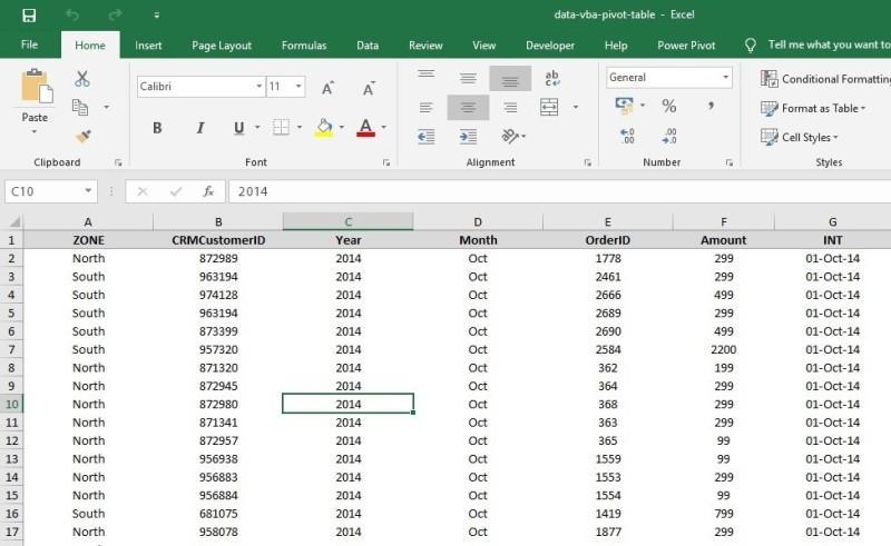
As you can see it is raw data, means there is no calculation or any sort of formatting just the plain data arranged in rows and columns. But one thing is worth noticing and should be bore in mind that the raw data must have headers that would best describe the data under it. There should not be multiple rows of header like the below example
(Image: 2)
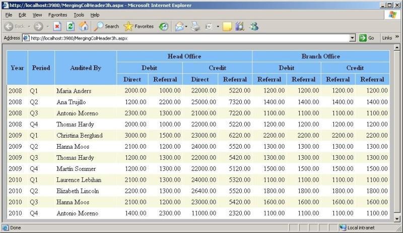
This table has got multiple rows of headers in blue colour
- Head Office, Branch Office
- Debit and Credit
- Direct, Referral.
In total there are three sets of headers. We need to normalize this data and bring single row of headers for every column like in (Image:1) that would not be obstacle in pivot table creation.
Now click on the Insert table, and you would see the option of Pivot table once you click on the option. The data on your current sheet would immediately get selected similar to image below
(Image:3)
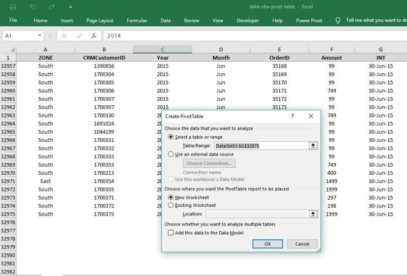
And a window would pop up showing various options to choose from, the pop up is asking the user to make the choice, by default “Select from a table or range” option is selected and, in the inputbox shows selection of your data.
The second option shows use of External data source, we will talk about that part later.
The third option ask you where you want to place the pivot table, it asking for the location. Whether the pivot table should be placed in new worksheet or the existing worksheet where the data is presently located. We would choose the first option i.e. the New worksheet so that it does not become chaotic to have both raw data and pivot table on the same sheet. And the last option is asking the user if he has multiple table and whether we want to add it to data model. In this article we are mainly concentrating on singular table so skip this option. We press OK button, with the default option selected in (Image:3)
(Image:4)
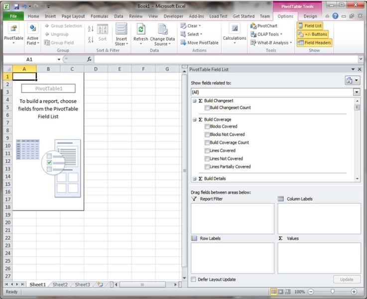
Along with the blank sheet we get a window on the right side, showing the columns that exist in our database on another worksheet. Our database or simply data is connected to this worksheet, it is showing the same columns. Now we can simply drag these columns in the four windows as the requirements demands. So, what exactly these four windows
The first window bears the name as “Report Filter”
Report Filter does the job of giving the options to choose from many. Once the choice is made the report automatically reflects the numbers with respect to the item selected in the list. The following picture will demonstrate the concept.
(Image:5)
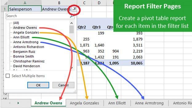
As you can see Sales person option is dragged in Report Filter window,” Salesperson” field name appears and beside this field name we get small symbol with a downward arrow mark encircled in red colour, as soon as we click on this symbol we get the drop down box from and there lies this item list from which we can make the choice and the report will reflect figures or data pertaining to the choice we have made from this list. To enable or disable the selection we need to simply click the option of “Select Multiple items” just above the “OK” button and then we can choose the item/items as per the requirement of the reports we are going to form.
The next three windows are for columns and rows and values.
We can simply drag the fields available in the above window into one of this three windows as per our requirement while the columns which contains numerical figures on which actual calculation needs to be done like sum, count, average, max, min can be easily performed without any formula so that saves punching of formula in the report formed by pivot tables. The option to cover additional formula can we can simply click on the arrow beside the field that has been dragged in the “Value” window by clicking on Value field settings. The following image will make it clearer to understand.


 0
0

