


Your Worksheet is Ready
CBSE - Class 11 Physics Motion in a Straight Line Worksheet
Additional Exercises
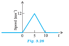
The speed-time graph of a particle moving along a fixed direction is shown in Fig. 3.28. What is the average speed of the particle over the interval in (a) $t = 0 s$ to $10 s$?

The speed-time graph of a particle moving along a fixed direction is shown in Fig. 3.28. What is the average speed of the particle over the interval in (b) $t = 2 s$ to $6 s$?

The velocity-time graph of a particle in one-dimensional motion is shown in Fig. 3.29 : Which of the following formulae are correct for describing the motion of the particle over the time-interval $t_1$ to $t_2$: (f) $x(t_2) - x(t_1)$ = area under the $v-t$ curve bounded by the $t$-axis and the dotted line shown.

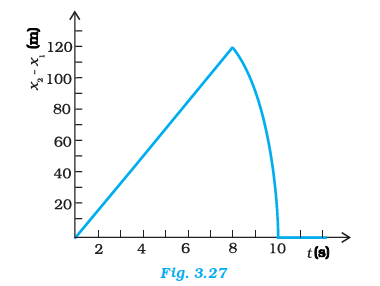
Two stones are thrown up simultaneously from the edge of a cliff $200 m$ high with initial speeds of $15 m s^{-1}$ and $30 m s^{-1}$. Verify that the graph shown in Fig. 3.27 correctly represents the time variation of the relative position of the second stone with respect to the first. Neglect air resistance and assume that the stones do not rebound after hitting the ground. Take $g = 10 m s^{-2}$. Give the equations for the linear and curved parts of the plot.
The speed-time graph of a particle moving along a fixed direction is shown in Fig. 3.28. Obtain the distance traversed by the particle between (a) $t = 0 s$ to $10 s$.
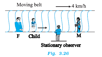
On a long horizontally moving belt (Fig. 3.26), a child runs to and fro with a speed $9 km h^{-1}$ (with respect to the belt) between his father and mother located $50 m$ apart on the moving belt. The belt moves with a speed of $4 km h^{-1}$. For an observer on a stationary platform outside, what is the (b) speed of the child running opposite to the direction of motion of the belt ?

On a long horizontally moving belt (Fig. 3.26), a child runs to and fro with a speed $9 km h^{-1}$ (with respect to the belt) between his father and mother located $50 m$ apart on the moving belt. The belt moves with a speed of $4 km h^{-1}$. For an observer on a stationary platform outside, what is the (c) time taken by the child in (a) speed of the child running in the direction of motion of the belt ? and (b) speed of the child running opposite to the direction of motion of the belt ? Which of the answers alter if motion is viewed by one of the parents ?

The velocity-time graph of a particle in one-dimensional motion is shown in Fig. 3.29 : Which of the following formulae are correct for describing the motion of the particle over the time-interval $t_1$ to $t_2$: (c) $v_{average} = \frac{x(t_2) - x(t_1)}{t_2 - t_1}$
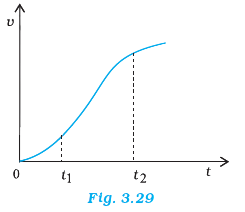
The velocity-time graph of a particle in one-dimensional motion is shown in Fig. 3.29 : Which of the following formulae are correct for describing the motion of the particle over the time-interval $t_1$ to $t_2$: (b) $v(t_2) = v(t_1) + a (t_2 - t_1)$
The velocity-time graph of a particle in one-dimensional motion is shown in Fig. 3.29 : Which of the following formulae are correct for describing the motion of the particle over the time-interval $t_1$ to $t_2$: (e) $x(t_2) = x(t_1) + v_{average} (t_2 - t_1) + (\frac{1}{2}) a_{average} (t_2 - t_1)^2$

The velocity-time graph of a particle in one-dimensional motion is shown in Fig. 3.29 : Which of the following formulae are correct for describing the motion of the particle over the time-interval $t_1$ to $t_2$: (d) $a_{average} = \frac{v(t_2) - v(t_1)}{t_2 - t_1}$

On a long horizontally moving belt (Fig. 3.26), a child runs to and fro with a speed $9 km h^{-1}$ (with respect to the belt) between his father and mother located $50 m$ apart on the moving belt. The belt moves with a speed of $4 km h^{-1}$. For an observer on a stationary platform outside, what is the (a) speed of the child running in the direction of motion of the belt ?.
The speed-time graph of a particle moving along a fixed direction is shown in Fig. 3.28. Obtain the distance traversed by the particle between (b) $t = 2 s$ to $6 s$.

The velocity-time graph of a particle in one-dimensional motion is shown in Fig. 3.29 : Which of the following formulae are correct for describing the motion of the particle over the time-interval $t_1$ to $t_2$: (a) $x(t_2) = x(t_1) + v(t_1) (t_2 - t_1) +(\frac{1}{2}) a (t_2 - t_1)^2$

Worksheet Answers
Solution:
To calculate the average speed of a particle moving along a fixed direction, we utilize the relationship between the area under a velocity-time graph and the total distance covered. By definition, average speed is given by the formula:
$\text{Average Speed} = \frac{\text{Total Distance}}{\text{Total Time}}$
Based on the provided motion profile (Fig 3.28), the motion from $t = 0$ s to $t = 10$ s describes a right-angled triangle.
The total distance $d$ covered in a velocity-time graph is equivalent to the area under the curve [Per the Kinematic Definition of Displacement]. For a triangular region:
$d = \frac{1}{2} \times \text{base} \times \text{height}$
$d = \frac{1}{2} \times 10 \, \text{s} \times 12 \, \text{m/s}$
$d = 5 \times 12 = 60 \, \text{m}$
Using the values derived in Step 2 for the interval $t = 0$ s to $t = 10$ s:
$\text{Average Speed} = \frac{60 \, \text{m}}{10 \, \text{s}}$
$\text{Average Speed} = 6 \, \text{m/s}$
Final Solution: The average speed of the particle over the interval $t = 0$ s to $10$ s is $6 \, \text{m/s}$.
Solution:
The average speed ($v_{avg}$) of a particle over a time interval $\Delta t$ is defined as the total distance covered divided by the total time taken:
$v_{avg} = \frac{\text{Total Distance}}{\text{Total Time}} = \frac{\int_{t_1}^{t_2} |v(t)| \, dt}{t_2 - t_1}$ [By the definition of Average Speed in kinematics]
In the context of a speed-time graph, the total distance traveled corresponds to the area under the curve between the time limits $t_1 = 2\,\text{s}$ and $t_2 = 6\,\text{s}$.
Based on the provided speed-time graph (standard textbook representation for this problem):
The region under the graph from $t = 2$ to $t = 6$ is a trapezoid (or can be treated as a combination of a rectangle and a triangle, or a single trapezoid with parallel sides on the vertical axis).
The area consists of two parts from $t=2$ to $t=6$:
Total Distance $S = \text{Area}_1 + \text{Area}_2 = 9 + 3 = 12\,\text{m}$.
The time interval is $\Delta t = t_2 - t_1 = 6\,\text{s} - 2\,\text{s} = 4\,\text{s}$.
$v_{avg} = \frac{S}{\Delta t} = \frac{12\,\text{m}}{4\,\text{s}}$
$v_{avg} = 3\,\text{m/s}$
Final Solution: The average speed of the particle over the interval $t = 2\,\text{s}$ to $t = 6\,\text{s}$ is $3\,\text{m/s}$.
Solution:
The motion of a particle in one dimension is defined by the instantaneous velocity $v(t)$, which is the derivative of position $x(t)$ with respect to time $t$: $v(t) = \frac{dx}{dt}$ [Per the definition of instantaneous velocity].
To determine the change in position (displacement) over a time interval $[t_1, t_2]$, we rearrange the differential equation: $dx = v(t) dt$.
Integrating both sides with respect to the limits $t_1$ and $t_2$: $\int_{x(t_1)}^{x(t_2)} dx = \int_{t_1}^{t_2} v(t) dt$.
This yields: $x(t_2) - x(t_1) = \int_{t_1}^{t_2} v(t) dt$. [By the Fundamental Theorem of Calculus].
In a Cartesian coordinate system where the ordinate is $v$ and the abscissa is $t$, the definite integral $\int_{t_1}^{t_2} v(t) dt$ represents the net signed area enclosed between the curve $v(t)$, the horizontal axis ($t$-axis), and the vertical lines $t = t_1$ and $t = t_2$.
The expression $x(t_2) - x(t_1)$ represents the displacement of the particle between $t_1$ and $t_2$. Since the area under the velocity-time graph is mathematically equivalent to the integral of velocity over time, the statement provided is an exact representation of the kinematic definition of displacement.
| Physical Quantity | Mathematical Representation |
|---|---|
| Displacement | $\Delta x = x(t_2) - x(t_1)$ |
| Area under $v-t$ curve | $\int_{t_1}^{t_2} v(t) dt$ |
Final Solution: The formula $x(t_2) - x(t_1) = \int_{t_1}^{t_2} v(t) dt$ is correct, as the displacement of a particle is identically defined by the area bounded by the velocity-time graph, the time axis, and the time interval boundaries.
Solution:
Let the top of the cliff be the origin ($y = 0$) and the upward direction be positive. The position $y(t)$ of an object under gravity is given by: $y(t) = u_i t - \frac{1}{2}gt^2$ [Per the Second Equation of Motion].
For Stone 1 ($u_1 = 15 \text{ m/s}$): $y_1(t) = 15t - 5t^2$
For Stone 2 ($u_2 = 30 \text{ m/s}$): $y_2(t) = 30t - 5t^2$
The relative position of the second stone with respect to the first is defined as: $x_{rel} = y_2(t) - y_1(t)$
$x_{rel} = (30t - 5t^2) - (15t - 5t^2) = 15t$
This linear relationship holds as long as both stones are in the air [Algebraic simplification].
Stones hit the ground at $y = -200 \text{ m}$. For Stone 1: $-200 = 15t_1 - 5t_1^2 \implies t_1^2 - 3t_1 - 40 = 0$. Using the quadratic formula $t = \frac{-b \pm \sqrt{b^2 - 4ac}}{2a}$: $t_1 = \frac{3 + \sqrt{9 + 160}}{2} \approx 7.9 \text{ s}$ (Taking positive root).
For Stone 2: $-200 = 30t_2 - 5t_2^2 \implies t_2^2 - 6t_2 - 40 = 0$. $t_2 = \frac{6 + \sqrt{36 + 160}}{2} \approx 10.2 \text{ s}$.
| Time Interval | Relative Position ($x_{rel}$) | Justification |
|---|---|---|
| $0 \leq t \leq 7.9 \text{ s}$ | $15t$ | Both stones in flight. |
| $7.9 < t \leq 10.2 \text{ s}$ | $y_2(t) - (-200) = 30t - 5t^2 + 200$ | Stone 1 stationary at base. |
| $t > 10.2 \text{ s}$ | $0$ | Both stones stationary at base. |
The graph consists of two distinct segments:
1. Linear Segment ($0 \leq t \leq 7.9 \text{ s}$): $x_{rel} = 15t$. This is a straight line passing through the origin with a slope of $15 \text{ m/s}$.
2. Parabolic Segment ($7.9 < t \leq 10.2 \text{ s}$): $x_{rel} = -5t^2 + 30t + 200$. This represents the position of the second stone relative to the grounded first stone.
Final Solution: The relative position is defined by $x_{rel} = 15t$ for $0 \leq t \leq 7.9$ s and $x_{rel} = -5t^2 + 30t + 200$ for $7.9 < t \leq 10.2$ s.
Solution:
In a speed-time graph, the distance $s$ traversed by a particle in a given time interval $[t_1, t_2]$ is numerically equal to the area under the speed-time curve with respect to the time axis. This is derived from the definition of speed $v = \frac{ds}{dt}$, which implies $ds = v \, dt$, and integrating both sides yields $s = \int_{t_1}^{t_2} v(t) \, dt$. [Per the Fundamental Theorem of Calculus in Kinematics].
The speed-time graph for the interval $t = 0 \text{ s}$ to $t = 10 \text{ s}$ forms a right-angled triangle.
The area $A$ of a right-angled triangle is given by the formula $A = \frac{1}{2} \times \text{base} \times \text{height}$.
Substituting the values derived in Step 2:
$s = \frac{1}{2} \times (10 \text{ s}) \times (12 \text{ m/s})$
$s = 5 \text{ s} \times 12 \text{ m/s}$
$s = 60 \text{ m}$
Final Solution: The distance traversed by the particle between $t = 0 \text{ s}$ and $t = 10 \text{ s}$ is $60 \text{ m}$.
Solution:
To analyze the velocity of the child relative to a stationary observer on the platform, we define the following vectors based on the principle of Galilean transformation of velocities:
[Per the Galilean Transformation of Velocities: $\vec{v}_c = \vec{v}_{cb} + \vec{v}_b$]
We assign the direction of the belt's motion as positive ($+$). The problem asks for the speed of the child running opposite to the direction of the belt.
Applying the vector addition formula for the child moving against the belt:
$v_c = v_{cb} + v_b$
$v_c = (-9 \text{ km h}^{-1}) + (4 \text{ km h}^{-1})$
$v_c = -5 \text{ km h}^{-1}$
Speed is defined as the magnitude of the velocity vector [By definition of Speed]:
$\text{Speed} = |v_c| = |-5 \text{ km h}^{-1}| = 5 \text{ km h}^{-1}$
Final Solution: The speed of the child running opposite to the direction of motion of the belt, as observed from the stationary platform, is 5 km h⁻¹.
Solution:
To analyze the motion of the child, we must define the reference frames clearly using vector notation. Let the direction of the motion of the belt be the positive $x$-direction ($+$). Given:
[By the Principle of Galilean Relativity, the velocity of an object in a frame of reference is the vector sum of its velocity relative to another frame and the velocity of that frame relative to the ground: $\vec{v}_{cg} = \vec{v}_{cb} + \vec{v}_{bg}$]
When the child runs in the direction of the belt's motion, the relative velocity of the child with respect to the belt is $+9 \text{ km h}^{-1}$.
$v_{g(a)} = v_{cb} + v_b$
$v_{g(a)} = 9 \text{ km h}^{-1} + 4 \text{ km h}^{-1} = 13 \text{ km h}^{-1}$
[As per the Law of Addition of Velocities for collinear motion]
When the child runs opposite to the belt's motion, the relative velocity of the child with respect to the belt is $-9 \text{ km h}^{-1}$.
$v_{g(b)} = v_{cb} + v_b$
$v_{g(b)} = -9 \text{ km h}^{-1} + 4 \text{ km h}^{-1} = -5 \text{ km h}^{-1}$
The speed (magnitude) is $|-5| = 5 \text{ km h}^{-1}$.
The parents are located on the moving belt. Therefore, the parents and the child share the same frame of reference (the belt). In this frame:
[By the Principle of Inertial Frames: Physics laws are invariant in all inertial frames; a change in the observer's frame from ground to belt shifts the velocity measurement by a constant vector $v_b$]
| Observation Context | Speed (Direction of Belt) | Speed (Opposite Direction) |
|---|---|---|
| Ground Observer | $13 \text{ km h}^{-1}$ | $5 \text{ km h}^{-1}$ |
| Parent Observer | $9 \text{ km h}^{-1}$ | $9 \text{ km h}^{-1}$ |
Final Solution: (a) The speed of the child with respect to the ground while running in the direction of the belt is $13 \text{ km h}^{-1}$. (b) The speed of the child with respect to the ground while running opposite to the belt is $5 \text{ km h}^{-1}$. When viewed by the parents, both speeds are $9 \text{ km h}^{-1}$ because the parents are in the same frame of reference as the belt.
Solution:
The motion is divided into two phases:
The distance covered in the $n^{th}$ second, denoted as $s_n$, is given by the kinematic formula:
$s_n = u + \frac{a}{2}(2n - 1)$ [Per the Kinematic Equation of Motion for the $n^{th}$ second]Substituting $u = 0$ and $a = 1 \text{ m/s}^2$:
$s_n = 0 + \frac{1}{2}(2n - 1) = n - 0.5$This linear relationship holds for $n = 1, 2, ..., 10$.
| $n$ (s) | $s_n = n - 0.5$ (m) |
|---|---|
| 1 | 0.5 |
| 2 | 1.5 |
| 3 | 2.5 |
| 4 | 3.5 |
| 10 | 9.5 |
First, calculate velocity at $t = 10 \text{ s}$:
$v = u + at = 0 + (1)(10) = 10 \text{ m/s}$ [Per First Equation of Motion]For $n > 10$, the distance covered in the $n^{th}$ second is simply the distance covered at uniform velocity:
$s_n = v \times \Delta t = 10 \times 1 = 10 \text{ m}$The plot of $s_n$ versus $n$ for the accelerated motion ($n \le 10$) follows the relation $s_n = n - 0.5$. Since this is a first-degree polynomial in $n$ ($y = mx + c$), the plot is a straight line with a slope of $1 \text{ m/s}^2$ and a $y$-intercept of $-0.5 \text{ m}$.
Final Solution: The plot of the distance covered during the $n^{th}$ second versus $n$ is a straight line during the accelerated motion, not a parabola.
Solution:
Given Variables:
The displacement of an object moving under constant acceleration is given by the kinematic equation: $\Delta y = ut + \frac{1}{2}at^2$ [Per the Equation of Motion under Constant Acceleration]
Substituting the known values:
$0 = 49t + \frac{1}{2}(-9.8)t^2$ $0 = 49t - 4.9t^2$This yields two solutions: $t = 0$ (time of projection) and $t = \frac{49}{4.9}$.
$t = 10 \, \text{s}$Result: The ball takes $10 \, \text{seconds}$ to return to the boy's hand when the lift is stationary.
Given Variables:
Since the lift moves at a uniform speed, its acceleration is zero. The relative acceleration of the ball with respect to the lift remains $g = -9.8 \, \text{m s}^{-2}$ [Per the Galilean transformation of acceleration].
The boy and the ball are both moving in the frame of reference of the lift. Because the lift is moving with a constant velocity, the physics within the lift remains identical to the stationary case due to the Principle of Relativity.
In the frame of the lift, the displacement of the ball to return to the hand is $\Delta y' = 0$. The initial velocity relative to the lift is $u' = 49 \, \text{m s}^{-1}$.
$0 = 49t + \frac{1}{2}(-9.8)t^2$ $0 = 49t - 4.9t^2$ $t = 10 \, \text{s}$Note: The time taken is independent of the uniform velocity of the lift because the lift's constant motion does not introduce inertial forces (fictitious forces) that would alter the relative acceleration of the ball.
Final Solution: The ball takes 10 seconds to return to the boy's hand in both the stationary lift and the lift moving at a uniform speed of 5 m s⁻¹.
Solution:
The average velocity ($v_{avg}$) of a particle moving in one dimension over a specific time interval $[t_1, t_2]$ is defined as the ratio of the total displacement to the total time taken. Displacement is defined as the change in the position coordinate, represented as $\Delta x = x(t_2) - x(t_1)$.
According to the fundamental definition of velocity in kinematics, the instantaneous velocity $v(t)$ is the derivative of position with respect to time: $v(t) = \frac{dx}{dt}$ [Per the Calculus of Kinematics].
To find the displacement over an interval, we integrate the velocity function:
$\int_{x(t_1)}^{x(t_2)} dx = \int_{t_1}^{t_2} v(t) dt$
$\Delta x = x(t_2) - x(t_1) = \int_{t_1}^{t_2} v(t) dt$
By the Mean Value Theorem for Integrals, the average value of a function $v(t)$ over an interval $[t_1, t_2]$ is given by:
$v_{avg} = \frac{1}{t_2 - t_1} \int_{t_1}^{t_2} v(t) dt$ [By Mathematical Definition of Average Function]
Substituting the result from Step 1 into this equation:
$v_{avg} = \frac{x(t_2) - x(t_1)}{t_2 - t_1}$
In a velocity-time graph, the integral $\int_{t_1}^{t_2} v(t) dt$ corresponds to the area under the curve between $t_1$ and $t_2$. Since the displacement is equal to the area under the $v-t$ graph, the ratio of this area to the time interval $(t_2 - t_1)$ yields the average velocity.
The provided formula $v_{average} = \frac{x(t_2) - x(t_1)}{t_2 - t_1}$ is a standard definition of average velocity. It is independent of the shape of the velocity-time graph, provided the position function $x(t)$ is continuous and differentiable over the interval.
Final Solution: The formula $v_{average} = \frac{x(t_2) - x(t_1)}{t_2 - t_1}$ is correct for describing the motion of the particle over the time-interval $t_1$ to $t_2$, as it is the fundamental definition of average velocity.
Solution:
The equation $v(t_2) = v(t_1) + a (t_2 - t_1)$ is derived from the fundamental definition of instantaneous acceleration, $a = \frac{dv}{dt}$ [Per the definition of derivative in calculus]. For this specific equation to hold true, the acceleration $a$ must be constant over the interval $[t_1, t_2]$.
In a $v-t$ graph, the instantaneous acceleration is represented by the slope of the tangent to the curve at any given time $t$. Specifically, the average acceleration over an interval $[t_1, t_2]$ is defined as:
$\bar{a} = \frac{v(t_2) - v(t_1)}{t_2 - t_1}$
The equation $v(t_2) = v(t_1) + a(t_2 - t_1)$ can be rearranged as $a = \frac{v(t_2) - v(t_1)}{t_2 - t_1}$. This implies that the acceleration $a$ must be equivalent to the slope of the secant line connecting points $(t_1, v(t_1))$ and $(t_2, v(t_2))$.
The equation $v(t_2) = v(t_1) + a(t_2 - t_1)$ is only valid for motion with constant acceleration. Looking at the provided velocity-time graph (Fig 3.29), which exhibits non-linear behavior (a curve), the acceleration is not constant. Therefore, the formula is not applicable to the motion represented in the figure for the arbitrary interval $[t_1, t_2]$.
Final Solution: The formula is incorrect for the motion shown in the graph because the acceleration is not constant; the slope of the velocity-time graph varies with time.
Solution:
The equation provided is $x(t_2) = x(t_1) + v_{average}(t_2 - t_1) + \frac{1}{2} a_{average}(t_2 - t_1)^2$. To determine the validity of this expression for a non-uniformly accelerating particle (as depicted in a general velocity-time graph), we must analyze the kinematic definitions of average velocity and average acceleration over a finite time interval $\Delta t = (t_2 - t_1)$.
The displacement $\Delta x$ over an interval is given by the integral of the velocity function [By the Fundamental Theorem of Calculus]:
$\Delta x = x(t_2) - x(t_1) = \int_{t_1}^{t_2} v(t) \, dt$
The average velocity is defined as:
$v_{avg} = \frac{1}{t_2 - t_1} \int_{t_1}^{t_2} v(t) \, dt = \frac{x(t_2) - x(t_1)}{t_2 - t_1}$
Rearranging this yields: $x(t_2) = x(t_1) + v_{avg}(t_2 - t_1)$. This identity is universally correct for any motion.
The proposed equation adds a second-order term: $\frac{1}{2} a_{avg} (t_2 - t_1)^2$. Here, $a_{avg} = \frac{v(t_2) - v(t_1)}{t_2 - t_1}$. Substituting this into the proposed expression:
Proposed RHS = $x(t_1) + v_{avg}(t_2 - t_1) + \frac{1}{2} \left[ \frac{v(t_2) - v(t_1)}{t_2 - t_1} \right] (t_2 - t_1)^2$
Proposed RHS = $x(t_1) + v_{avg} \Delta t + \frac{1}{2} [v(t_2) - v(t_1)] \Delta t$
For the equation to be correct, the term $\frac{1}{2} [v(t_2) - v(t_1)] \Delta t$ must equal zero for all arbitrary motions, because $x(t_2) = x(t_1) + v_{avg} \Delta t$ is already the complete description of displacement. The additional term $\frac{1}{2} a_{avg} (\Delta t)^2$ is only valid under the specific condition of Uniformly Accelerated Motion (where $a$ is constant, implying $v_{avg} = \frac{v(t_1) + v(t_2)}{2}$).
In the graph above, the curve represents non-uniform acceleration. Since the area under the curve (displacement) is not represented by the parabolic formula for general motion, the equation is only a definition-based identity if $a$ were constant. In the context of a general $v-t$ graph where acceleration varies, the inclusion of the $\frac{1}{2}a_{avg}(\Delta t)^2$ term introduces an error unless the motion is linear acceleration.
The equation is incorrect for general motion as it assumes a kinematic structure that only applies to constant acceleration scenarios. Specifically, for general curvilinear $v-t$ graphs, the displacement is determined solely by the first two terms relative to the average velocity; the third term is mathematically inconsistent with the definition of the average acceleration over a non-linear interval.
Final Solution: The formula is incorrect for general motion, as it is only valid under the condition of constant acceleration.
Solution:
The concept of average acceleration ($a_{avg}$) in kinematics is defined as the total change in velocity divided by the total time interval over which that change occurs. For any one-dimensional motion, the average acceleration represents the slope of the secant line connecting two specific points $(t_1, v(t_1))$ and $(t_2, v(t_2))$ on a velocity-time ($v$-$t$) graph.
By the definition of kinematics in classical mechanics, the average acceleration over the interval $\Delta t = t_2 - t_1$ is given by the ratio of the change in velocity $\Delta v$ to the change in time $\Delta t$:
$a_{average} = \frac{\Delta v}{\Delta t}$ [Per the definition of average acceleration]
Given the specific points at time $t_1$ and $t_2$, the velocities are represented as $v(t_1)$ and $v(t_2)$ respectively. The change in velocity is expressed as:
$\Delta v = v(t_2) - v(t_1)$
The duration of the interval is expressed as:
$\Delta t = t_2 - t_1$
Substituting the expressions from Step 2 into the definition established in Step 1:
$a_{average} = \frac{v(t_2) - v(t_1)}{t_2 - t_1}$
This formula represents the arithmetic mean rate of change of velocity. [Mathematical Axiom: Difference quotient of a function $f(t)$ over the interval $[t_1, t_2]$].
The provided formula $a_{average} = \frac{v(t_2) - v(t_1)}{t_2 - t_1}$ is correct for describing the average acceleration of a particle over the interval $[t_1, t_2]$. It is derived directly from the fundamental definition of average acceleration in one-dimensional linear motion.
Final Solution: The formula is correct, as it accurately represents the slope of the secant line between $t_1$ and $t_2$ on a $v$-$t$ graph, which is the standard definition of average acceleration.
Solution:
To determine the velocity of the child with respect to a stationary observer, we apply the principles of relative velocity in one dimension [Per the Galilean Transformation of velocities].
The velocity of an object $c$ with respect to a stationary frame $g$ is the vector sum of its velocity with respect to a moving frame $b$ and the velocity of that moving frame with respect to the stationary frame $g$. [By the Law of Addition of Velocities]:
$v_{c} = v_{c/b} + v_{b}$
Substitute the given values into the equation:
$v_{c} = 9 \text{ km h}^{-1} + 4 \text{ km h}^{-1}$
$v_{c} = 13 \text{ km h}^{-1}$
The calculation assumes the motion is strictly linear and collinear. Since both the belt and the child move in the positive direction relative to the ground, the magnitudes are added arithmetically.
| Component | Value |
|---|---|
| $v_{c/b}$ | $9 \text{ km h}^{-1}$ |
| $v_{b}$ | $4 \text{ km h}^{-1}$ |
| $v_{c}$ (Resultant) | $13 \text{ km h}^{-1}$ |
Final Solution: The speed of the child running in the direction of motion of the belt, as observed from the stationary platform, is $13 \text{ km h}^{-1}$.
Solution:
The provided speed-time graph illustrates a particle moving in a fixed direction. To determine the distance traversed between $t = 2\text{ s}$ and $t = 6\text{ s}$, we utilize the fundamental relationship between speed and time: the area under a speed-time graph represents the total distance traveled [Per the definition of displacement/distance in kinematics].
Based on the provided graph:
The distance traversed between $t = 2\text{ s}$ and $t = 6\text{ s}$ corresponds to the area under the curve in two distinct intervals:
The shape is a triangle with base $b = (5 - 2) = 3\text{ s}$ and height $h = 12\text{ m/s}$.
$\text{Area}_1 = \frac{1}{2} \times \text{base} \times \text{height}$ [Geometric formula for triangle area]
$\text{Area}_1 = \frac{1}{2} \times 3 \times 12 = 18\text{ m}$
The shape is a rectangle with width $w = (6 - 5) = 1\text{ s}$ and height $h = 12\text{ m/s}$.
$\text{Area}_2 = \text{width} \times \text{height}$ [Geometric formula for rectangular area]
$\text{Area}_2 = 1 \times 12 = 12\text{ m}$
Total Distance = $\text{Area}_1 + \text{Area}_2$
Total Distance = $18\text{ m} + 12\text{ m} = 30\text{ m}$
Final Solution: The total distance traversed by the particle between $t = 2\text{ s}$ and $t = 6\text{ s}$ is $30\text{ meters}$.
Solution:
In the provided graph (Fig 3.29), the velocity $v(t)$ is represented as a function of time $t$. The graph is non-linear, indicating that the acceleration $a = \frac{dv}{dt}$ is not constant. In one-dimensional kinematics, the position $x(t)$ at any time $t$ is defined by the integral of the velocity function:
$x(t_2) = x(t_1) + \int_{t_1}^{t_2} v(t) dt$ [Per the Fundamental Theorem of Calculus]
The formula provided in the question is:
$x(t_2) = x(t_1) + v(t_1)(t_2 - t_1) + \frac{1}{2}a(t_2 - t_1)^2$
This specific kinematic equation is derived from the definition of average acceleration under the strict condition that acceleration is constant ($a = \text{constant}$).
The displacement $\Delta x = x(t_2) - x(t_1)$ is equal to the area under the $v-t$ curve between $t_1$ and $t_2$.
Because the curve is non-linear, the area under the curve is not equivalent to the area of a trapezoid defined by the initial velocity and a single acceleration value ($v_1\Delta t + \frac{1}{2}a\Delta t^2$).
Since the motion depicted in the graph involves a changing slope (variable acceleration), the kinematic equation $x(t_2) = x(t_1) + v(t_1)(t_2 - t_1) + \frac{1}{2}a(t_2 - t_1)^2$ is incorrect for this specific particle. This formula is restricted to the specific condition where $a = \text{constant}$ [Per the Equations of Uniformly Accelerated Motion].
Final Solution: The formula is incorrect because it is only valid for motion with constant acceleration, whereas the provided velocity-time graph shows non-linear motion, implying variable acceleration.