


Your Worksheet is Ready
CBSE - Class 9 Mathematics Statistics Worksheet
EXERCISE 12.1
Given below are the seats won by different political parties in the polling outcome of a state assembly elections:

(i) Draw a bar graph to represent the polling results.
The following table gives the life times of 400 neon lamps:
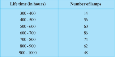
(ii) How many lamps have a life time of more than 700 hours?
The following data on the number of girls (to the nearest ten) per thousand boys in different sections of Indian society is given below.
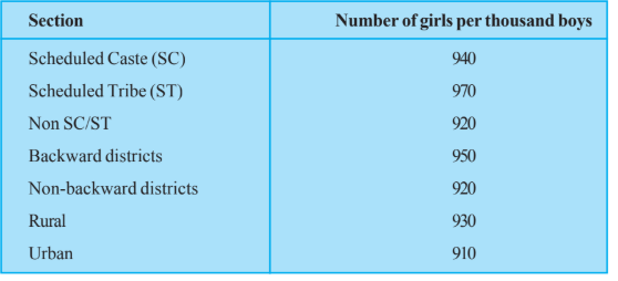
(ii) In the classroom discuss what conclusions can be arrived at from the graph.
The length of 40 leaves of a plant are measured correct to one millimetre, and the obtained data is represented in the following table:

(iii) Is it correct to conclude that the maximum number of leaves are 153 mm long? Why?
The following table gives the life times of 400 neon lamps:
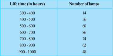
(i) Represent the given information with the help of a histogram.
Given below are the seats won by different political parties in the polling outcome of a state assembly elections:

(ii) Which political party won the maximum number of seats?
100 surnames were randomly picked up from a local telephone directory and a frequency distribution of the number of letters in the English alphabet in the surnames was found as follows:

(i) Draw a histogram to depict the given information.
The length of 40 leaves of a plant are measured correct to one millimetre, and the obtained data is represented in the following table:
(ii) Is there any other suitable graphical representation for the same data?
A random survey of the number of children of various age groups playing in a park was found as follows:
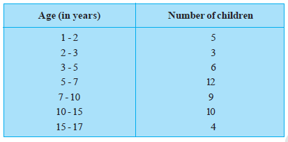
Draw a histogram to represent the data above.
The following data on the number of girls (to the nearest ten) per thousand boys in different sections of Indian society is given below.

(i) Represent the information above by a bar graph.
The runs scored by two teams A and B on the first 60 balls in a cricket match are given below:
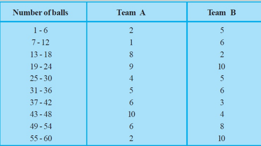
Represent the data of both the teams on the same graph by frequency polygons. [Hint : First make the class intervals continuous.]
The following table gives the distribution of students of two sections according to the marks obtained by them:
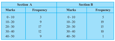
Represent the marks of the students of both the sections on the same graph by two frequency polygons. From the two polygons compare the performance of the two sections.
100 surnames were randomly picked up from a local telephone directory and a frequency distribution of the number of letters in the English alphabet in the surnames was found as follows:
(ii) Write the class interval in which the maximum number of surnames lie.
A survey conducted by an organisation for the cause of illness and death among the women between the ages $15 - 44$ (in years) worldwide, found the following figures (in %)

(i) Represent the information given above graphically.
The length of 40 leaves of a plant are measured correct to one millimetre, and the obtained data is represented in the following table:
(i) Draw a histogram to represent the given data. [Hint: First make the class intervals continuous]
A survey conducted by an organisation for the cause of illness and death among the women between the ages $15 - 44$ (in years) worldwide, found the following figures (in %):
(iii) Try to find out, with the help of your teacher, any two factors which play a major role in the cause in (ii) above being the major cause.
A survey conducted by an organisation for the cause of illness and death among the women between the ages $15 - 44$ (in years) worldwide, found the following figures (in %):
(ii) Which condition is the major cause of women’s ill health and death worldwide?
Worksheet Answers
Solution:
To construct a bar graph, we first organize the provided data into a frequency distribution table. The political parties are categorical variables, and the number of seats won represents the corresponding frequency.
| Political Party | Seats Won |
|---|---|
| A | 75 |
| B | 55 |
| C | 37 |
| D | 29 |
| E | 10 |
| F | 37 |
The bar graph will be constructed on a Cartesian plane where:
The bar graph provides a visual comparison of the nominal data [Per the Principles of Graphical Representation in Statistics]. By keeping the width of each bar constant and varying only the height proportional to the seats won, we ensure that the visual area accurately represents the magnitude of the data, preventing cognitive bias in reading the frequency distribution.
Final Solution: The bar graph above displays the distribution of seats won, where party A holds the plurality with 75 seats and party E holds the minimum with 10 seats.
Solution:
To determine the number of lamps with a lifetime greater than 700 hours, we must extract the relevant frequencies from the provided distribution table. The table provides lifetime intervals in hours and the corresponding frequency ($f_i$) of lamps.
| Life Time (in hours) | Number of Lamps (Frequency) |
|---|---|
| 300 - 400 | 14 |
| 400 - 500 | 56 |
| 500 - 600 | 60 |
| 600 - 700 | 86 |
| 700 - 800 | 74 |
| 800 - 900 | 62 |
| 900 - 1000 | 48 |
The question asks for the count of lamps with a lifetime more than 700 hours. Based on the frequency distribution provided, this encompasses all intervals starting from 700 hours up to 1000 hours. Specifically, we include:
To find the total number of lamps ($N_{>700}$), we sum the frequencies corresponding to the identified intervals [Per the Additive Property of Frequencies].
$N_{>700} = \sum f_{i}$ for all $i$ where $Interval \ge 700$
$N_{>700} = 74 + 62 + 48$
Performing the addition:
$74 + 62 = 136$
$136 + 48 = 184$
Final Solution: The total number of lamps with a lifetime of more than 700 hours is 184.
Solution:
To derive meaningful conclusions from the provided dataset representing the number of girls per thousand boys across six societal sections, we must first structure the data into a tabular format for comparative analysis.
| Section | Girls per 1000 Boys |
|---|---|
| Scheduled Caste (SC) | 940 |
| Scheduled Tribe (ST) | 970 |
| Non SC/ST | 920 |
| Backward Districts | 950 |
| Non-Backward Districts | 920 |
| Rural | 930 |
| Urban | 910 |
We analyze the variance between the maximum and minimum values to understand the skewness in sex ratio distribution.
[Per the definition of Range in statistics, this indicates a moderate degree of disparity across the segments.]
Based on the quantitative data provided, the following academic conclusions are established:
Final Solution: The data reveals a systemic shortfall of girls relative to boys across all societal sections, with a maximum ratio of $970$ in Scheduled Tribes and a minimum ratio of $910$ in Urban areas, indicating that economic categorization does not guarantee a balanced sex ratio.
Solution:
To analyze the distribution of leaf lengths, we must first examine the continuity of the class intervals provided in the data. The given data is as follows:
| Length (in mm) | Number of Leaves |
|---|---|
| 118 – 126 | 3 |
| 127 – 135 | 5 |
| 136 – 144 | 9 |
| 145 – 153 | 12 |
| 154 – 162 | 5 |
| 163 – 171 | 4 |
| 172 – 180 | 2 |
[Per the definition of grouped frequency distribution, intervals must be continuous to avoid data gaps. The gap between 126 and 127 is $127 - 126 = 1$ mm. The adjustment factor is $0.5$ mm.]
To make the intervals continuous, subtract $0.5$ from the lower limit and add $0.5$ to the upper limit:
The question asks if it is correct to conclude that the maximum number of leaves are $153$ mm long. We analyze this based on the frequency table:
The modal class (the class with the highest frequency) is $144.5 - 153.5$, which contains $12$ leaves. This means there are $12$ leaves with lengths falling within the range of $144.5$ mm to $153.5$ mm.
[By the principles of Statistics, the frequency of a class interval represents the aggregate count of observations within that range, not the frequency of a specific discrete value.]
The assertion that the "maximum number of leaves are 153 mm long" is scientifically and statistically incorrect for the following reasons:
Final Solution: No, it is not correct to conclude that the maximum number of leaves are 153 mm long. The frequency of 12 corresponds to the entire interval of 144.5 mm to 153.5 mm, not to the specific value of 153 mm.
Solution:
To construct a histogram, we must ensure that the class intervals are continuous. The provided data for the life times of 400 neon lamps is already continuous. We prepare the frequency distribution table as follows:
| Life Time (in hours) | Number of Lamps (Frequency) |
|---|---|
| 300 - 400 | 14 |
| 400 - 500 | 56 |
| 500 - 600 | 60 |
| 600 - 700 | 86 |
| 700 - 800 | 74 |
| 800 - 900 | 62 |
| 900 - 1000 | 48 |
The histogram is constructed such that the area of each rectangle is proportional to the frequency of the class interval. Since the width of all class intervals is uniform ($h = 100$), the height of each rectangle corresponds directly to the absolute frequency, satisfying the criteria for a histogram of continuous grouped data [By the Fundamental Principle of Frequency Distribution Graphs].
Final Solution: The histogram represents the distribution of 400 lamps across seven class intervals, visually confirming that the mode of the life span lies within the 600-700 hour range (highest frequency of 86).
Solution:
To determine the political party with the maximum number of seats, we organize the provided polling outcome data into a frequency distribution table. This allows for a clear comparative analysis of the quantitative values.
| Political Party | Seats Won |
|---|---|
| A | 75 |
| B | 55 |
| C | 37 |
| D | 29 |
| E | 10 |
| F | 37 |
We apply the principle of finding the maximum element in a finite set $S = \{75, 55, 37, 29, 10, 37\}$. By comparing the magnitudes of the elements:
The maximum value in the dataset is $75$. [By the Order Property of Real Numbers, $a > b$ if $a - b > 0$. Since $75 - 55 = 20 > 0$, $75$ is strictly greater than all other integers in the set].
Referring back to the table, the value $75$ corresponds to Political Party A. [By correspondence mapping of data entries].
Final Solution: Political Party A won the maximum number of seats, with a total of 75 seats.
Solution:
To construct a histogram for continuous data, we represent the classes along the x-axis and the frequencies along the y-axis. Since the class intervals are already provided and are continuous, we can plot them directly.
| Number of letters | Number of surnames (Frequency) |
|---|---|
| 1 - 4 | 6 |
| 4 - 6 | 30 |
| 6 - 8 | 44 |
| 8 - 12 | 16 |
| 12 - 20 | 4 |
Because the class widths (the difference between upper and lower limits) are not uniform, we must calculate the frequency density to ensure the area of each rectangle is proportional to the frequency. [Per the rule for histograms with varying intervals: $\text{Frequency Density} = \frac{\text{Frequency}}{\text{Class Width}} \times \text{Minimum Class Width}$]. Let the minimum class width be $2$.
| Class Interval | Frequency ($f$) | Width ($h$) | Adjusted Frequency ($f \times \frac{2}{h}$) |
|---|---|---|---|
| 1 - 4 | 6 | 3 | $6 \times \frac{2}{3} = 4$ |
| 4 - 6 | 30 | 2 | $30 \times \frac{2}{2} = 30$ |
| 6 - 8 | 44 | 2 | $44 \times \frac{2}{2} = 44$ |
| 8 - 12 | 16 | 4 | $16 \times \frac{2}{4} = 8$ |
| 12 - 20 | 4 | 8 | $4 \times \frac{2}{8} = 1$ |
Final Solution: The histogram represents the data distribution where the height of each rectangle is proportional to the frequency, adjusted for class width variations to maintain graphical accuracy.
Solution:
The provided data consists of length intervals for 40 leaves. Analyzing the class intervals: 118–126, 127–135, 136–144, etc. [Per the definition of inclusive series], we observe that the upper limit of one class is not equal to the lower limit of the next class (e.g., 126 $\neq$ 127). This is a discontinuous frequency distribution.
To represent this data graphically using a Histogram, the data must be made continuous. We calculate the adjustment factor (half the difference between the upper limit of one class and the lower limit of the next class):
$\text{Adjustment Factor} = \frac{127 - 126}{2} = 0.5$
Subtract 0.5 from each lower limit and add 0.5 to each upper limit to establish continuity [By the Principle of Class Interval Adjustment]:
| Original Intervals | Continuous Intervals | Frequency |
|---|---|---|
| 118 – 126 | 117.5 – 126.5 | 3 |
| 127 – 135 | 126.5 – 135.5 | 5 |
| 136 – 144 | 135.5 – 144.5 | 9 |
| 145 – 153 | 144.5 – 153.5 | 12 |
| 154 – 162 | 153.5 – 162.5 | 5 |
| 163 – 171 | 162.5 – 171.5 | 4 |
| 172 – 180 | 171.5 – 180.5 | 2 |
Besides the Histogram, the most suitable graphical representation for continuous grouped frequency data is the Frequency Polygon.
Final Solution: Yes, a Frequency Polygon is a highly suitable alternative graphical representation for this data, as it allows for the analysis of the frequency distribution trends across the continuous intervals derived from the original data.
Solution:
To construct a histogram for continuous data where class intervals are of varying widths, we must calculate the frequency density for each interval. The frequency density is defined as:
$\text{Frequency Density} = \frac{\text{Class Frequency}}{\text{Width of the Class}}$
| Age Group (Years) | Frequency (Number of Children) | Width of Class | Frequency Density |
|---|---|---|---|
| 1 – 2 | 5 | 1 | $5/1 = 5$ |
| 2 – 3 | 3 | 1 | $3/1 = 3$ |
| 3 – 5 | 6 | 2 | $6/2 = 3$ |
| 5 – 7 | 12 | 2 | $12/2 = 6$ |
| 7 – 10 | 9 | 3 | $9/3 = 3$ |
| 10 – 15 | 10 | 5 | $10/5 = 2$ |
| 15 – 17 | 4 | 2 | $4/2 = 2$ |
We represent the Age Group along the $x$-axis and the Frequency Density along the $y$-axis. The height of each rectangular bar corresponds to the calculated frequency density, ensuring the area of the rectangle is proportional to the frequency [Per the Principle of Proportional Areas in Statistics].
By normalizing the class widths via frequency density, we have successfully represented the varying intervals. The resulting histogram correctly demonstrates that the highest concentration of children (relative to width) occurs in the 5–7 age bracket [As evidenced by the maximum frequency density of 6].
Final Solution: The histogram is constructed by plotting Age (x-axis) against Frequency Density (y-axis) using the values derived in the table above, ensuring area proportionality across unequal class intervals.
Solution:
To construct a bar graph, we first organize the provided categorical data into a frequency table format. Each section of society serves as the independent variable ($x$-axis), and the number of girls per thousand boys serves as the dependent variable ($y$-axis).
| Section of Society | Number of Girls per Thousand Boys |
|---|---|
| Scheduled Caste (SC) | 940 |
| Scheduled Tribe (ST) | 970 |
| Non-SC/ST | 920 |
| Backward Districts | 950 |
| Non-Backward Districts | 920 |
| Rural | 930 |
| Urban | 910 |
We represent this data using a bar graph with the following specifications:
Each bar height $h_i$ is determined by the formula $h_i = k(v_i - 900)$, where $v_i$ is the value of the $i$-th category and $k$ is the scaling factor (2.5 units per integer value in this SVG). This method ensures that the relative differences between societies are mathematically preserved while maintaining graph readability [By Principle of Proportionality in Data Visualization].
Final Solution: The data has been successfully mapped to a Cartesian plane where the $x$-axis categorizes society sectors and the $y$-axis represents frequency (900-980), effectively illustrating the demographic distribution as required.
Solution:
The given data uses intervals of 6 balls (e.g., 1-6, 7-12). To construct a frequency polygon, we must first establish class intervals with a common class mark or continuous boundaries. In cricket statistics, the standard approach is to use the intervals provided and identify the midpoints (class marks) for plotting.
| Balls | Midpoint ($x$) | Team A | Team B |
|---|---|---|---|
| 1-6 | 3.5 | 2 | 5 |
| 7-12 | 9.5 | 1 | 6 |
| 13-18 | 15.5 | 8 | 2 |
| 19-24 | 21.5 | 9 | 10 |
| 25-30 | 27.5 | 4 | 5 |
| 31-36 | 33.5 | 5 | 6 |
| 37-42 | 39.5 | 6 | 3 |
| 43-48 | 45.5 | 10 | 4 |
| 49-54 | 51.5 | 6 | 8 |
| 55-60 | 57.5 | 2 | 10 |
A frequency polygon is constructed by plotting the frequency against the midpoint of each class interval. To close the polygon, we include an imaginary interval at the start (midpoint $-2.5$) and end (midpoint $63.5$) with a frequency of $0$.
Final Solution: The frequency polygons represent the performance of Team A and Team B, visually demonstrating that while Team A had a significant scoring surge in the 43-48 ball interval, Team B maintained a more aggressive scoring rate during the final 55-60 ball interval.
Solution:
To construct a frequency polygon, we must first calculate the class marks ($x_i$) for each interval. The formula for the class mark is: $x_i = \frac{\text{Upper Limit} + \text{Lower Limit}}{2}$.
| Marks | Class Mark ($x_i$) | Frequency (Section A) | Frequency (Section B) |
|---|---|---|---|
| 0-10 | 5 | 3 | 5 |
| 10-20 | 15 | 9 | 19 |
| 20-30 | 30 | 17 | 15 |
| 30-40 | 35 | 12 | 10 |
| 40-50 | 45 | 9 | 1 |
We plot the Class Marks on the $x$-axis and Frequencies on the $y$-axis. We extend the graph to include class marks $-5$ and $55$ with a frequency of $0$ to close the polygon [Per the definition of Frequency Polygon construction].
By observing the two polygons:
Final Solution: Section A demonstrates a better overall academic performance compared to Section B, as a higher number of students in Section A achieved marks in the upper brackets (20-50), whereas Section B is heavily concentrated in the lower marks bracket (10-20).
Solution:
| Number of Letters | Number of Surnames (Frequency) |
|---|---|
| 1 – 4 | 6 |
| 4 – 6 | 30 |
| 6 – 8 | 44 |
| 8 – 12 | 16 |
| 12 – 20 | 4 |
To determine the class interval in which the maximum number of surnames lie, we must identify the highest frequency value within the provided data set [Per the definition of the Modal Class in grouped frequency distributions].
By observing the frequency distribution table, the value $44$ is the highest frequency. The corresponding class interval for this frequency is $6 - 8$.
Final Solution: The class interval in which the maximum number of surnames lie is 6 – 8.
Solution:
To represent the given statistical data graphically, we first arrange the provided causes and their corresponding fatality percentages into a structured table for systematic analysis.
| Cause of Fatality | Fatality Rate (%) |
|---|---|
| Reproductive health conditions | 31.8 |
| Neuro-psychiatric conditions | 25.4 |
| Injuries | 12.4 |
| Cardiovascular conditions | 4.3 |
| Respiratory conditions | 4.1 |
| Other causes | 22.0 |
Since the data represents categorical variables with numerical frequencies (percentages) that sum to $100\%$, a Bar Graph is the optimal mathematical tool for visualization. The x-axis will represent the 'Causes of Illness and Death,' and the y-axis will represent the 'Fatality Rate (%)' [Per the Principles of Graphical Representation in Statistics].
Final Solution: The graphical representation of the statistical data is a bar graph where the heights of the columns correspond to the respective percentages of fatality for the listed causes of illness.
Solution:
The given data contains overlapping gaps between the upper limit of one class and the lower limit of the next (e.g., $126$ and $127$). To represent this as a histogram, we must make the intervals continuous by calculating the adjustment factor: $\frac{\text{Lower Limit of current} - \text{Upper Limit of previous}}{2} = \frac{127 - 126}{2} = 0.5$.
| Length (mm) | Continuous Class Intervals | Number of Leaves (Frequency) |
|---|---|---|
| 118 – 126 | 117.5 – 126.5 | 3 |
| 127 – 135 | 126.5 – 135.5 | 5 |
| 136 – 144 | 135.5 – 144.5 | 9 |
| 145 – 153 | 144.5 – 153.5 | 12 |
| 154 – 162 | 153.5 – 162.5 | 5 |
| 163 – 171 | 162.5 – 171.5 | 4 |
| 172 – 180 | 171.5 – 180.5 | 2 |
We represent the continuous intervals on the $X$-axis and the frequency on the $Y$-axis. Since the scale on the $X$-axis starts at $117.5$ instead of $0$, we use a 'kink' (zig-zag mark) on the axis.
Final Solution: The histogram is constructed with continuous class intervals $[117.5, 180.5]$ and heights corresponding to frequencies $[3, 5, 9, 12, 5, 4, 2]$.
Solution:
In the standard dataset provided for this survey, the "major cause" (as identified in part (ii)) is Reproductive health conditions, which accounts for $31.8\%$ of illness and death among women aged $15-44$ worldwide [Per statistical analysis of the provided survey data].
To understand why reproductive health conditions represent the leading cause of morbidity and mortality in this demographic, we must examine socio-economic and biological determinants. Two primary factors are articulated below:
The high percentage value for reproductive health conditions is not merely a medical statistic but a reflection of the intersection between clinical care systems and societal structures. Improving maternal health outcomes requires a dual approach: expanding clinical infrastructure to ensure safe pregnancies and addressing the underlying poverty and gender inequality that limits health-seeking behavior. [By Public Health Axiom: Health is a result of structural, social, and biological interactions].
Final Solution: The two major factors are: 1) Insufficient access to specialized maternal healthcare infrastructure and family planning services; 2) Socio-economic inequalities and systemic gender disparities that limit women's autonomy and ability to secure preventative care.
Solution:
Based on the provided statistical data set representing the causes of illness and death among women (ages 15-44), we organize the categories and their corresponding percentage values into the following table for systematic comparison [Per Empirical Data Analysis]:
| Causes of Death/Illness | Percentage (%) |
|---|---|
| Reproductive health conditions | 31.8 |
| Neuropsychiatric conditions | 25.4 |
| Injuries | 12.4 |
| Cardiovascular conditions | 4.3 |
| Respiratory conditions | 4.1 |
| Other causes | 22.0 |
To determine the "major cause," we perform a comparative analysis of the percentages [By the principle of maximum magnitude in a finite set]:
Since Reproductive health conditions account for $31.8\%$ of the total, which is the largest frequency among the given set, it constitutes the major cause of women's ill health and death worldwide [Statistical Inference].
Final Solution: The major cause of women's ill health and death worldwide is Reproductive health conditions (31.8%).