Your Worksheet is Ready
CBSE - Class 10 Mathematics Statistics Worksheet
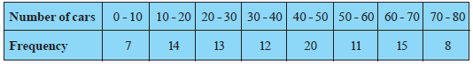
A student noted the number of cars passing through a spot on a road for 100 periods each of 3 minutes and summarised it in the table given below. Find the mode of the data:
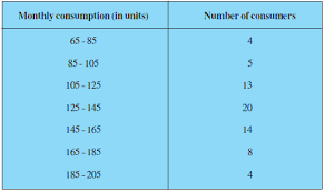
The following frequency distribution gives the monthly consumption of electricity of 68 consumers of a locality. Find the median, mean and mode of the data and compare them.
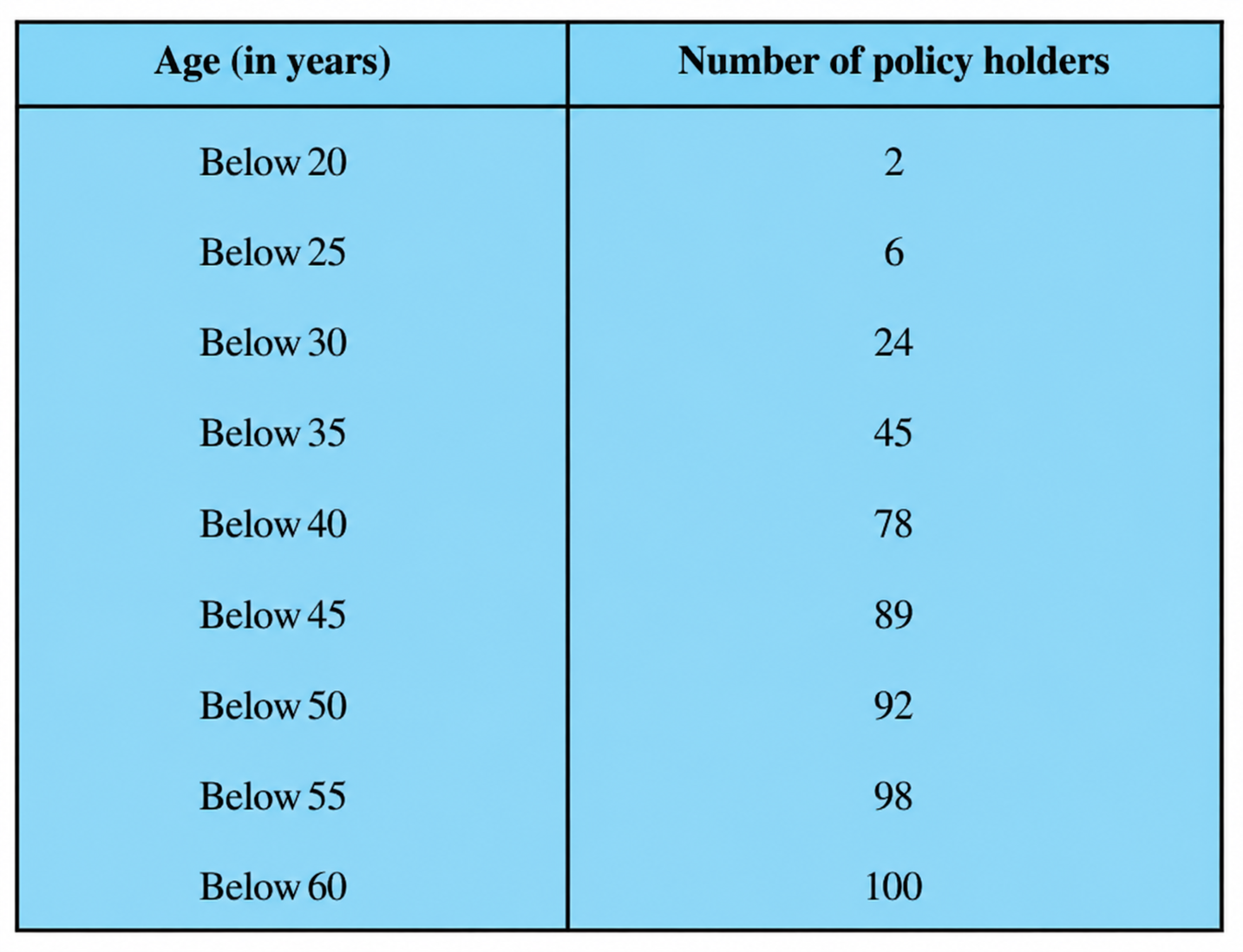
A life insurance agent found the following data for distribution of ages of 100 policy holders. Calculate the median age, if policies are given only to persons having age 18 years onwards but less than 60 year.
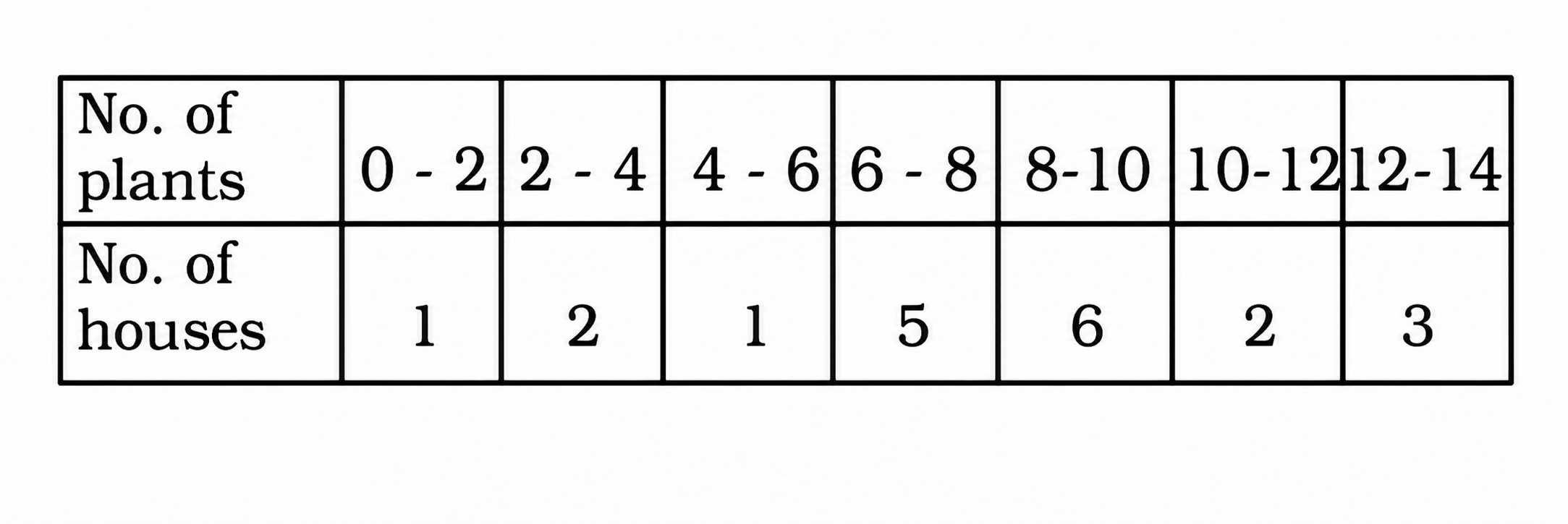
A survey was conducted by a group of students as a part of their environment awareness programme, in which they collected the following data regarding the number of plants in 20 houses in a locality. Find the mean number of plants per house.
Which method did you use for finding the mean, and why?
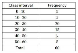
If the median of the distribution given below is 28.5, find the values of $x$ and $y$.
The lengths of 40 leaves of a plant are measured correct to the nearest millimetre, and the data obtained is represented in the following table :
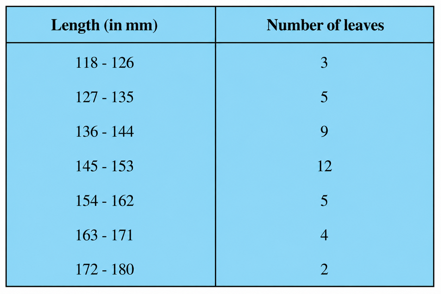
Find the median length of the leaves. (Hint : The data needs to be converted to continuous classes for finding the median, since the formula assumes continuous classes. The classes then change to 117.5 - 126.5, 126.5 - 135.5, . . ., 171.5 - 180.5.)
The following table shows the ages of the patients admitted in a hospital during a year:
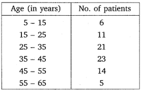
Find the mode and the mean of the data given above. Compare and interpret the two measures of central tendency.
The following data gives the information on the observed lifetimes (in hours) of 225 electrical components :
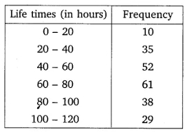
Determine the modal lifetimes of the components.
The following table gives the distribution of the life time of 400 neon lamps :
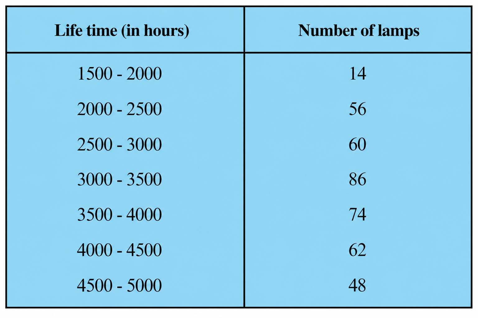
Find the median life time of a lamp.
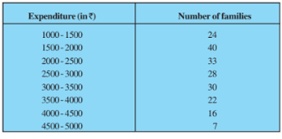
The following data gives the distribution of total monthly household expenditure of 200 families of a village. Find the modal monthly expenditure of the families. Also, find the mean monthly expenditure :
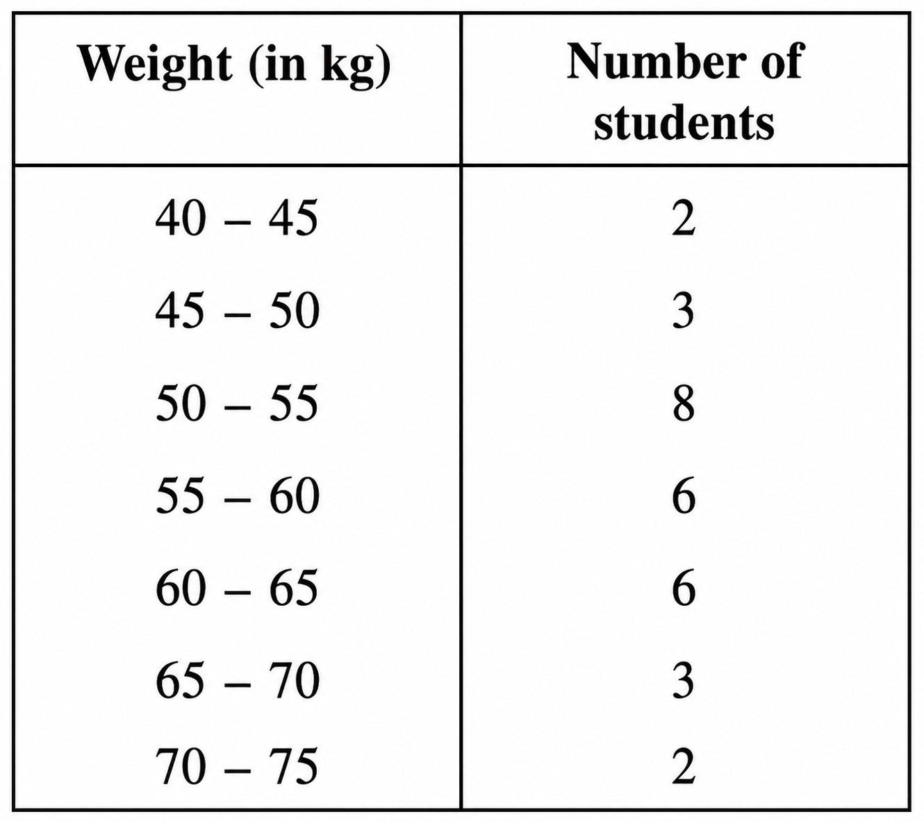
The distribution below gives the weights of 30 students of a class. Find the median weight of the students.
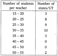
The following distribution gives the state-wise teacher-student ratio in higher secondary schools of India. Find the mode and mean of this data. Interpret the two measures.
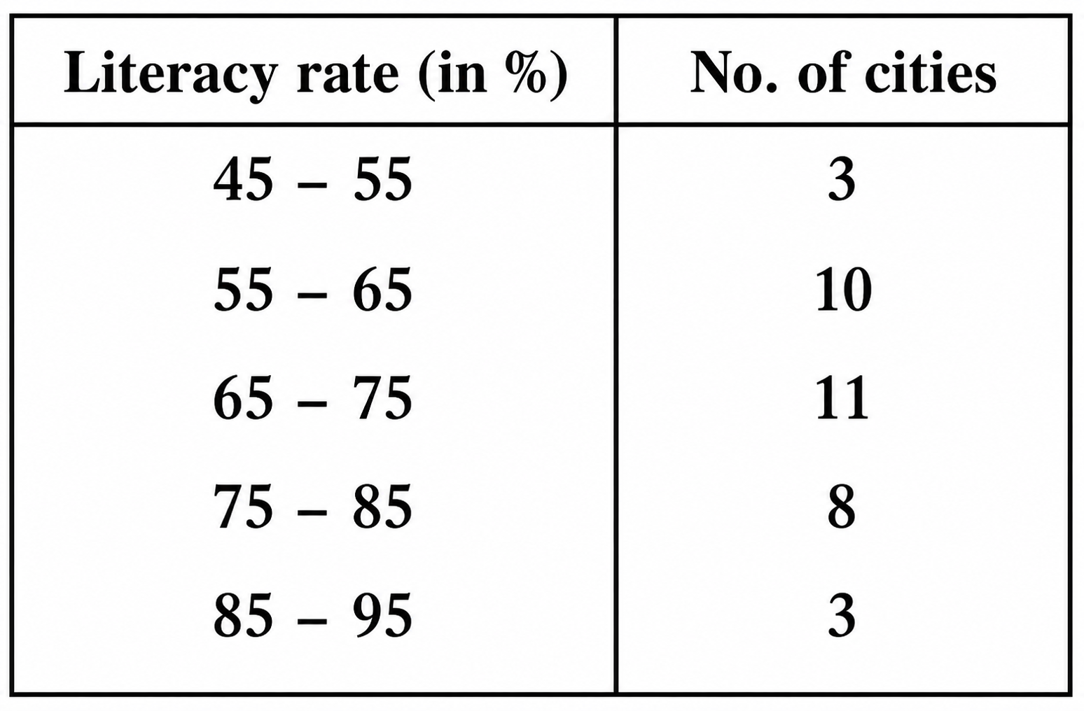
The following table gives the literacy rate (in percentage) of 35 cities. Find the mean literacy rate.
Consider the following distribution of daily wages of 50 workers of a factory.
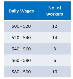
Find the mean daily wages of the workers of the factory by using an appropriate method.
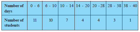
A class teacher has the following absentee record of 40 students of a class for the whole term. Find the mean number of days a student was absent.
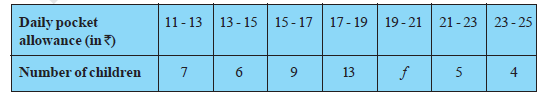
The following distribution shows the daily pocket allowance of children of a locality. The mean pocket allowance is Rs 18. Find the missing frequency $f$.
To find out the concentration of $SO_2$ in the air (in parts per million, i.e., ppm), the data was collected for 30 localities in a certain city and is presented below:
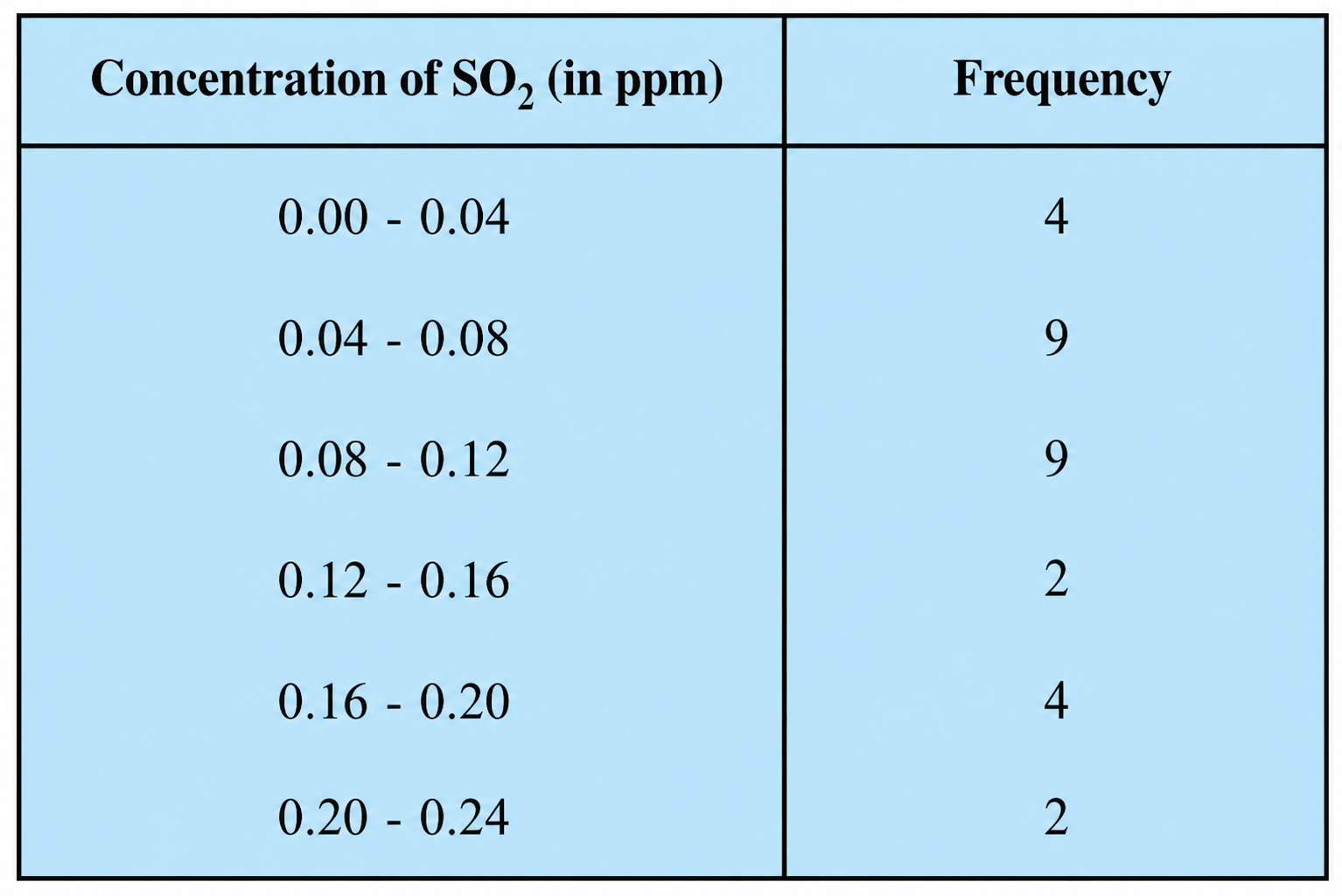
Find the mean concentration of $SO_2$ in the air.
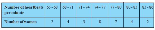
Thirty women were examined in a hospital by a doctor and the number of heartbeats per minute were recorded and summarised as follows. Find the mean heartbeats per minute for these women, choosing a suitable method.
The table below shows the daily expenditure on food of 25 households in a locality.
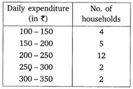
Find the mean daily expenditure on food by a suitable method.
In a retail market, fruit vendors were selling mangoes kept in packing boxes. These boxes contained varying number of mangoes. The following was the distribution of mangoes according to the number of boxes.
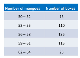
Find the mean number of mangoes kept in a packing box. Which method of finding the mean did you choose?
Worksheet Answers
Solution:
Given: A frequency distribution table representing the number of cars passing through a spot in 100 periods of 3 minutes each.
| Number of cars | Frequency ($f_i$) |
|---|---|
| 0 - 10 | 7 |
| 10 - 20 | 14 |
| 20 - 30 | 13 |
| 30 - 40 | 12 |
| 40 - 50 | 20 |
| 50 - 60 | 11 |
| 60 - 70 | 15 |
| 70 - 80 | 8 |
To find: The mode of the given grouped frequency distribution.
Step 1: Identify the Modal Class
The modal class is the class interval with the highest frequency. Observing the table, the highest frequency is $20$, which corresponds to the class interval $40 - 50$.
Therefore, the Modal Class is $40 - 50$.
Step 2: State the Formula for Mode
The formula for calculating the mode of grouped data is:
$\text{Mode} = l + \left( \frac{f_1 - f_0}{2f_1 - f_0 - f_2} \right) \times h$
Where:
Step 3: Extract the Variables
Based on the modal class $40 - 50$:
Step 4: Substitute and Calculate
Substituting the values into the formula:
$\text{Mode} = 40 + \left( \frac{20 - 12}{2(20) - 12 - 11} \right) \times 10$
$\text{Mode} = 40 + \left( \frac{8}{40 - 23} \right) \times 10$
$\text{Mode} = 40 + \left( \frac{8}{17} \right) \times 10$
$\text{Mode} = 40 + \frac{80}{17}$
Performing the division: $80 \div 17 \approx 4.7058...$
$\text{Mode} = 40 + 4.71$ (rounded to two decimal places)
$\text{Mode} = 44.71$
Final Answer: The mode of the data is 44.71 cars.
Solution:
Given: A frequency distribution table representing the monthly electricity consumption (in units) of 68 consumers.
| Monthly Consumption (units) | Number of Consumers ($f_i$) |
|---|---|
| 65 - 85 | 4 |
| 85 - 105 | 5 |
| 105 - 125 | 13 |
| 125 - 145 | 20 |
| 145 - 165 | 14 |
| 165 - 185 | 8 |
| 185 - 205 | 4 |
To Find: The Mean, Median, and Mode of the given data and compare them.
Step 1: Calculation of Mean ($\bar{x}$) using the Step-Deviation Method
Let the assumed mean $a = 135$. The class size $h = 20$.
| Class Interval | Frequency ($f_i$) | Class Mark ($x_i$) | $d_i = x_i - 135$ | $u_i = \frac{d_i}{20}$ | $f_i u_i$ |
|---|---|---|---|---|---|
| 65-85 | 4 | 75 | -60 | -3 | -12 |
| 85-105 | 5 | 95 | -40 | -2 | -10 |
| 105-125 | 13 | 115 | -20 | -1 | -13 |
| 125-145 | 20 | 135 | 0 | 0 | 0 |
| 145-165 | 14 | 155 | 20 | 1 | 14 |
| 165-185 | 8 | 175 | 40 | 2 | 16 |
| 185-205 | 4 | 195 | 60 | 3 | 12 |
| Total | $\sum f_i = 68$ | - | - | - | $\sum f_i u_i = 7$ |
Formula for Mean: $\bar{x} = a + \left( \frac{\sum f_i u_i}{\sum f_i} \right) \times h$
$\bar{x} = 135 + \left( \frac{7}{68} \right) \times 20 = 135 + \frac{140}{68} \approx 135 + 2.06 = 137.06$
Step 2: Calculation of Median
Cumulative Frequency ($cf$) table:
| Class Interval | Frequency ($f_i$) | Cumulative Frequency ($cf$) |
|---|---|---|
| 65-85 | 4 | 4 |
| 85-105 | 5 | 9 |
| 105-125 | 13 | 22 |
| 125-145 | 20 | 42 |
| 145-165 | 14 | 56 |
| 165-185 | 8 | 64 |
| 185-205 | 4 | 68 |
Here, $n = 68$, so $\frac{n}{2} = 34$. The cumulative frequency just greater than 34 is 42, which corresponds to the class 125-145.
Median Class = 125-145. Lower limit ($l$) = 125, $f = 20$, $cf$ of preceding class = 22, $h = 20$.
Median = $l + \left( \frac{\frac{n}{2} - cf}{f} \right) \times h = 125 + \left( \frac{34 - 22}{20} \right) \times 20 = 125 + 12 = 137$.
Step 3: Calculation of Mode
The maximum frequency is 20, which corresponds to the class 125-145. This is the Modal Class.
$l = 125, f_1 = 20, f_0 = 13, f_2 = 14, h = 20$.
Mode = $l + \left( \frac{f_1 - f_0}{2f_1 - f_0 - f_2} \right) \times h = 125 + \left( \frac{20 - 13}{2(20) - 13 - 14} \right) \times 20$
Mode = $125 + \left( \frac{7}{40 - 27} \right) \times 20 = 125 + \left( \frac{7}{13} \right) \times 20 = 125 + 10.77 = 135.77$.
Step 4: Comparison
Mean $\approx 137.06$, Median $= 137$, Mode $\approx 135.77$.
The values are very close to each other, indicating a nearly symmetric distribution.
Final Answer: Mean = 137.06 units, Median = 137 units, Mode = 135.77 units.
Solution:
Given: The frequency distribution of ages of 100 policy holders, provided as a cumulative frequency table (less than type):
| Age (years) | Number of policy holders (Cumulative Frequency) |
|---|---|
| Below 20 | 2 |
| Below 25 | 6 |
| Below 30 | 24 |
| Below 35 | 45 |
| Below 40 | 78 |
| Below 45 | 89 |
| Below 50 | 92 |
| Below 55 | 98 |
| Below 60 | 100 |
To Find: The median age of the policy holders.
Step 1: Convert the cumulative frequency distribution into a standard frequency distribution table.
To calculate the median, we need the class intervals and their corresponding frequencies ($f_i$).
| Class Interval | Frequency ($f_i$) | Cumulative Frequency ($cf$) |
|---|---|---|
| 15-20 | 2 | 2 |
| 20-25 | 6 - 2 = 4 | 6 |
| 25-30 | 24 - 6 = 18 | 24 |
| 30-35 | 45 - 24 = 21 | 45 |
| 35-40 | 78 - 45 = 33 | 78 |
| 40-45 | 89 - 78 = 11 | 89 |
| 45-50 | 92 - 89 = 3 | 92 |
| 50-55 | 98 - 92 = 6 | 98 |
| 55-60 | 100 - 98 = 2 | 100 |
| Total | $N = 100$ | - |
Step 2: Identify the median class.
The total number of observations is $N = 100$.
We calculate $\frac{N}{2} = \frac{100}{2} = 50$.
Looking at the cumulative frequency column, the first cumulative frequency greater than 50 is 78, which corresponds to the class interval 35-40.
Therefore, the median class is 35-40.
Step 3: Apply the Median Formula.
The formula for the median of a grouped frequency distribution is:
$\text{Median} = l + \left( \frac{\frac{N}{2} - cf}{f} \right) \times h$
Where:
Step 4: Perform the calculation.
Substitute the values into the formula:
$\text{Median} = 35 + \left( \frac{50 - 45}{33} \right) \times 5$
$\text{Median} = 35 + \left( \frac{5}{33} \right) \times 5$
$\text{Median} = 35 + \frac{25}{33}$
$\text{Median} = 35 + 0.7575...$
$\text{Median} \approx 35.76$
Final Answer: The median age of the policy holders is 35.76 years.
Solution:
Given: A frequency distribution table representing the number of plants in 20 houses.
| Number of plants | 0-2 | 2-4 | 4-6 | 6-8 | 8-10 | 10-12 | 12-14 |
|---|---|---|---|---|---|---|---|
| Number of houses ($f_i$) | 1 | 2 | 1 | 5 | 6 | 2 | 3 |
To Find: The mean number of plants per house and the justification for the chosen method.
Step 1: Choosing the Method
Since the class intervals are small and the frequencies are manageable, we will use the Direct Method to calculate the mean. The formula for the mean ($\bar{x}$) using the direct method is:
$\bar{x} = \frac{\sum f_i x_i}{\sum f_i}$
where $x_i$ is the class mark of each interval.
Step 2: Constructing the Calculation Table
We calculate the class mark ($x_i$) for each interval using the formula: $x_i = \frac{\text{Upper Limit} + \text{Lower Limit}}{2}$.
| Number of plants (Class Interval) | Number of houses ($f_i$) | Class mark ($x_i$) | $f_i \times x_i$ |
|---|---|---|---|
| 0-2 | 1 | 1 | 1 |
| 2-4 | 2 | 3 | 6 |
| 4-6 | 1 | 5 | 5 |
| 6-8 | 5 | 7 | 35 |
| 8-10 | 6 | 9 | 54 |
| 10-12 | 2 | 11 | 22 |
| 12-14 | 3 | 13 | 39 |
| Total | $\sum f_i = 20$ | - | $\sum f_i x_i = 162$ |
Step 3: Calculating the Mean
Using the values obtained from the table:
$\sum f_i = 20$
$\sum f_i x_i = 1 + 6 + 5 + 35 + 54 + 22 + 39 = 162$
Substituting these into the mean formula:
$\bar{x} = \frac{162}{20}$
$\bar{x} = 8.1$
Step 4: Justification
The Direct Method was used because the numerical values of the class marks ($x_i$) and the frequencies ($f_i$) are small, making the multiplication $f_i x_i$ straightforward and easy to compute without the need for complex deviations or assumed mean methods.
Final Answer: The mean number of plants per house is 8.1.
Solution:
Given: A frequency distribution table with a total frequency $N = 60$ and a median value of $28.5$.
| Class Interval | Frequency ($f$) |
|---|---|
| 0-10 | 5 |
| 10-20 | $x$ |
| 20-30 | 20 |
| 30-40 | 15 |
| 40-50 | $y$ |
| 50-60 | 5 |
| Total | 60 |
To find: The values of $x$ and $y$.
Step 1: Constructing the Cumulative Frequency Table
| Class Interval | Frequency ($f$) | Cumulative Frequency ($cf$) |
|---|---|---|
| 0-10 | 5 | 5 |
| 10-20 | $x$ | $5 + x$ |
| 20-30 | 20 | $25 + x$ |
| 30-40 | 15 | $40 + x$ |
| 40-50 | $y$ | $40 + x + y$ |
| 50-60 | 5 | $45 + x + y$ |
Step 2: Establishing the first linear equation
Since the total frequency is given as $60$, we have:
$45 + x + y = 60$Step 3: Identifying the Median Class
The median is given as $28.5$. Since $28.5$ lies between $20$ and $30$, the median class is $20-30$.
From the median class $20-30$:
Step 4: Applying the Median Formula
The formula for the median is: $\text{Median} = l + \left( \frac{\frac{N}{2} - cf}{f} \right) \times h$
Substituting the known values:
$28.5 = 20 + \left( \frac{30 - (5 + x)}{20} \right) \times 10$Step 5: Solving for $y$
Substitute $x = 8$ into Equation 1:
$8 + y = 15$Final Answer: The values are $x = 8$ and $y = 7$.
Solution:
Given: The frequency distribution of the lengths of 40 leaves measured to the nearest millimetre.
| Length (mm) | Number of leaves ($f$) |
|---|---|
| 118 - 126 | 3 |
| 127 - 135 | 5 |
| 136 - 144 | 9 |
| 145 - 153 | 12 |
| 154 - 162 | 5 |
| 163 - 171 | 4 |
| 172 - 180 | 2 |
To Find: The median length of the leaves.
Step 1: Converting to Continuous Classes
The given classes are discontinuous (e.g., 126 and 127). To make them continuous, we subtract 0.5 from the lower limit and add 0.5 to the upper limit of each class interval.
| Class Interval | Frequency ($f$) | Cumulative Frequency ($cf$) |
|---|---|---|
| 117.5 - 126.5 | 3 | 3 |
| 126.5 - 135.5 | 5 | 8 |
| 135.5 - 144.5 | 9 | 17 |
| 144.5 - 153.5 | 12 | 29 |
| 153.5 - 162.5 | 5 | 34 |
| 162.5 - 171.5 | 4 | 38 |
| 171.5 - 180.5 | 2 | 40 |
| Total | $n = 40$ | - |
Step 2: Identifying the Median Class
The total number of observations is $n = 40$.
We calculate $\frac{n}{2} = \frac{40}{2} = 20$.
Looking at the cumulative frequency column, the first cumulative frequency greater than 20 is 29, which corresponds to the class interval $144.5 - 153.5$.
Thus, the median class is $144.5 - 153.5$.
Step 3: Applying the Median Formula
The formula for the median is:
$\text{Median} = l + \left( \frac{\frac{n}{2} - cf}{f} \right) \times h$
Where:
$l$ (lower limit of median class) = $144.5$
$n$ (total number of observations) = $40$
$cf$ (cumulative frequency of the class preceding the median class) = $17$
$f$ (frequency of the median class) = $12$
$h$ (class size) = $153.5 - 144.5 = 9$
Step 4: Calculation
$\text{Median} = 144.5 + \left( \frac{20 - 17}{12} \right) \times 9$
$\text{Median} = 144.5 + \left( \frac{3}{12} \right) \times 9$
$\text{Median} = 144.5 + \left( \frac{1}{4} \right) \times 9$
$\text{Median} = 144.5 + 2.25$
$\text{Median} = 146.75$
Final Answer: The median length of the leaves is 146.75 mm.
Solution:
Given: The frequency distribution of ages of patients admitted to a hospital:
| Age (in years) | 5-15 | 15-25 | 25-35 | 35-45 | 45-55 | 55-65 |
|---|---|---|---|---|---|---|
| Number of patients ($f_i$) | 6 | 11 | 21 | 23 | 14 | 5 |
To Find: The Mode and the Mean of the given data, and to compare and interpret the results.
Formula: $\text{Mode} = l + \left( \frac{f_1 - f_0}{2f_1 - f_0 - f_2} \right) \times h$
Where:
Step 1.1: Identify the Modal Class. The maximum frequency is $23$, which corresponds to the class interval $35-45$. Thus, the modal class is $35-45$.
Step 1.2: Assign values. $l = 35$, $f_1 = 23$, $f_0 = 21$, $f_2 = 14$, $h = 10$.
Step 1.3: Substitute into the formula.
$\text{Mode} = 35 + \left( \frac{23 - 21}{2(23) - 21 - 14} \right) \times 10$
$\text{Mode} = 35 + \left( \frac{2}{46 - 35} \right) \times 10 = 35 + \left( \frac{2}{11} \right) \times 10 = 35 + \frac{20}{11} \approx 35 + 1.818 = 36.82$
Step 2.1: Prepare the table for Assumed Mean Method ($A = 40$).
| Age | $f_i$ | Class Mark ($x_i$) | $d_i = x_i - 40$ | $f_i d_i$ |
|---|---|---|---|---|
| 5-15 | 6 | 10 | -30 | -180 |
| 15-25 | 11 | 20 | -20 | -220 |
| 25-35 | 21 | 30 | -10 | -210 |
| 35-45 | 23 | 40 | 0 | 0 |
| 45-55 | 14 | 50 | 10 | 140 |
| 55-65 | 5 | 60 | 20 | 100 |
| Total | 80 | - | - | -370 |
Step 2.2: Apply the Mean formula.
$\text{Mean} (\bar{x}) = A + \frac{\sum f_i d_i}{\sum f_i} = 40 + \left( \frac{-370}{80} \right) = 40 - 4.625 = 35.375$
The modal age is approximately $36.82$ years, representing the age group with the highest number of patients admitted. The mean age is $35.38$ years, representing the average age of all patients admitted. Since the mean is slightly less than the mode, it indicates that the distribution is slightly negatively skewed, but both measures suggest that the majority of patients admitted are in the mid-30s age range.
Final Answer: The Mode is 36.82 years and the Mean is 35.38 years.
Solution:
Given: The frequency distribution of the lifetimes (in hours) of 225 electrical components is as follows:
| Lifetimes (hours) | 0-20 | 20-40 | 40-60 | 60-80 | 80-100 | 100-120 |
|---|---|---|---|---|---|---|
| Frequency ($f_i$) | 10 | 35 | 52 | 61 | 38 | 29 |
To Find: The modal lifetime of the electrical components.
Step 1: Identifying the Modal Class
The modal class is the class interval with the highest frequency. Looking at the frequency distribution table, the highest frequency is $61$, which corresponds to the class interval $60-80$.
Therefore, the Modal Class is $60-80$.
Step 2: Stating the Formula for Mode
The formula for calculating the mode of a grouped frequency distribution is:
$\text{Mode} = l + \left( \frac{f_1 - f_0}{2f_1 - f_0 - f_2} \right) \times h$
Where:
$l$ = Lower limit of the modal class
$h$ = Size of the class interval
$f_1$ = Frequency of the modal class
$f_0$ = Frequency of the class preceding the modal class
$f_2$ = Frequency of the class succeeding the modal class
Step 3: Extracting the Values
From the given data:
$l = 60$
$h = 80 - 60 = 20$
$f_1 = 61$
$f_0 = 52$
$f_2 = 38$
Step 4: Substituting Values into the Formula
$\text{Mode} = 60 + \left( \frac{61 - 52}{2(61) - 52 - 38} \right) \times 20$
[Substituting the identified values into the formula]
Step 5: Performing the Arithmetic Calculations
$\text{Mode} = 60 + \left( \frac{9}{122 - 90} \right) \times 20$
$\text{Mode} = 60 + \left( \frac{9}{32} \right) \times 20$
$\text{Mode} = 60 + \left( \frac{180}{32} \right)$
$\text{Mode} = 60 + 5.625$
$\text{Mode} = 65.625$
Final Answer: The modal lifetime of the electrical components is 65.625 hours.
Solution:
Given: The frequency distribution of the lifetime of 400 neon lamps as follows:
| Lifetime (hours) | Number of Lamps ($f_i$) |
|---|---|
| 1500 - 2000 | 14 |
| 2000 - 2500 | 56 |
| 2500 - 3000 | 60 |
| 3000 - 3500 | 86 |
| 3500 - 4000 | 74 |
| 4000 - 4500 | 62 |
| 4500 - 5000 | 48 |
To Find: The median lifetime of the neon lamps.
Step 1: Construct the Cumulative Frequency Table
To find the median, we first calculate the cumulative frequency ($cf$) for each class interval.
| Lifetime (hours) | Frequency ($f_i$) | Cumulative Frequency ($cf$) |
|---|---|---|
| 1500 - 2000 | 14 | 14 |
| 2000 - 2500 | 56 | 70 |
| 2500 - 3000 | 60 | 130 |
| 3000 - 3500 | 86 | 216 |
| 3500 - 4000 | 74 | 290 |
| 4000 - 4500 | 62 | 352 |
| 4500 - 5000 | 48 | 400 |
| Total | $N = 400$ | - |
Step 2: Identify the Median Class
The total number of observations is $N = 400$.
We calculate $\frac{N}{2} = \frac{400}{2} = 200$.
Looking at the cumulative frequency column, the first cumulative frequency greater than 200 is 216, which corresponds to the class interval $3000 - 3500$.
Therefore, the median class is $3000 - 3500$.
Step 3: Apply the Median Formula
The formula for the median of a grouped frequency distribution is:
$\text{Median} = l + \left( \frac{\frac{N}{2} - cf}{f} \right) \times h$
Where:
$l$ (lower limit of median class) = $3000$
$N$ (total frequency) = $400$
$cf$ (cumulative frequency of the class preceding the median class) = $130$
$f$ (frequency of the median class) = $86$
$h$ (class size) = $500$
Step 4: Perform the Calculation
Substitute the values into the formula:
$\text{Median} = 3000 + \left( \frac{200 - 130}{86} \right) \times 500$
$\text{Median} = 3000 + \left( \frac{70}{86} \right) \times 500$
$\text{Median} = 3000 + \left( \frac{35000}{86} \right)$ [Simplifying the fraction: $\frac{70}{86} = \frac{35}{43}$]
$\text{Median} = 3000 + 406.9767...$
$\text{Median} \approx 3406.98$
Final Answer: The median lifetime of a lamp is 3406.98 hours.
Solution:
Given: The frequency distribution of monthly household expenditure of 200 families.
| Expenditure (in ₹) | Number of Families ($f_i$) |
|---|---|
| 1000 - 1500 | 24 |
| 1500 - 2000 | 40 |
| 2000 - 2500 | 33 |
| 2500 - 3000 | 28 |
| 3000 - 3500 | 30 |
| 3500 - 4000 | 22 |
| 4000 - 4500 | 16 |
| 4500 - 5000 | 7 |
To Find: The Modal monthly expenditure and the Mean monthly expenditure.
Step 1: Identify the Modal Class. The modal class is the class interval with the highest frequency. Here, the highest frequency is $40$, which corresponds to the class interval $1500 - 2000$.
Step 2: Apply the Mode Formula. The formula for mode is: $Mode = l + \left( \frac{f_1 - f_0}{2f_1 - f_0 - f_2} \right) \times h$
Where:
$l$ (lower limit of modal class) = $1500$
$f_1$ (frequency of modal class) = $40$
$f_0$ (frequency of class preceding modal class) = $24$
$f_2$ (frequency of class succeeding modal class) = $33$
$h$ (class size) = $500$
Step 3: Calculation.
$Mode = 1500 + \left( \frac{40 - 24}{2(40) - 24 - 33} \right) \times 500$
$Mode = 1500 + \left( \frac{16}{80 - 57} \right) \times 500$
$Mode = 1500 + \left( \frac{16}{23} \right) \times 500$
$Mode = 1500 + \frac{8000}{23} \approx 1500 + 347.83 = 1847.83$
Step 1: Calculate Class Marks ($x_i$). $x_i = \frac{\text{Upper Limit} + \text{Lower Limit}}{2}$. Let assumed mean $a = 2750$.
| Expenditure | $f_i$ | $x_i$ | $d_i = x_i - 2750$ | $u_i = \frac{d_i}{500}$ | $f_i u_i$ |
|---|---|---|---|---|---|
| 1000-1500 | 24 | 1250 | -1500 | -3 | -72 |
| 1500-2000 | 40 | 1750 | -1000 | -2 | -80 |
| 2000-2500 | 33 | 2250 | -500 | -1 | -33 |
| 2500-3000 | 28 | 2750 | 0 | 0 | 0 |
| 3000-3500 | 30 | 3250 | 500 | 1 | 30 |
| 3500-4000 | 22 | 3750 | 1000 | 2 | 44 |
| 4000-4500 | 16 | 4250 | 1500 | 3 | 48 |
| 4500-5000 | 7 | 4750 | 2000 | 4 | 28 |
| Total | 200 | - | - | - | -35 |
Step 2: Apply the Step-Deviation Formula. $\bar{x} = a + \left( \frac{\sum f_i u_i}{\sum f_i} \right) \times h$
$\bar{x} = 2750 + \left( \frac{-35}{200} \right) \times 500$
$\bar{x} = 2750 + (-0.175 \times 500)$
$\bar{x} = 2750 - 87.5 = 2662.5$
Final Answer: The modal monthly expenditure is ₹1847.83 and the mean monthly expenditure is ₹2662.50.
Solution:
Given: A frequency distribution of the weights of 30 students.
| Weight (kg) | Number of students (f) |
|---|---|
| 40 - 45 | 2 |
| 45 - 50 | 3 |
| 50 - 55 | 8 |
| 55 - 60 | 6 |
| 60 - 65 | 6 |
| 65 - 70 | 3 |
| 70 - 75 | 2 |
To Find: The median weight of the students.
Step 1: Constructing the Cumulative Frequency Table
To find the median, we must first calculate the cumulative frequency ($cf$) for each class interval.
| Weight (kg) | Frequency ($f$) | Cumulative Frequency ($cf$) |
|---|---|---|
| 40 - 45 | 2 | 2 |
| 45 - 50 | 3 | 2 + 3 = 5 |
| 50 - 55 | 8 | 5 + 8 = 13 |
| 55 - 60 | 6 | 13 + 6 = 19 |
| 60 - 65 | 6 | 19 + 6 = 25 |
| 65 - 70 | 3 | 25 + 3 = 28 |
| 70 - 75 | 2 | 28 + 2 = 30 |
| Total | $n = 30$ | - |
Step 2: Identifying the Median Class
The total number of observations is $n = 30$.
We calculate $\frac{n}{2} = \frac{30}{2} = 15$.
[The median class is the class interval whose cumulative frequency is greater than or nearest to $\frac{n}{2}$.]
Looking at the table, the cumulative frequency just greater than 15 is 19, which corresponds to the class interval 55 - 60.
Step 3: Applying the Median Formula
The formula for the median is:
$Median = l + \left( \frac{\frac{n}{2} - cf}{f} \right) \times h$
Where:
$l$ (lower limit of median class) = $55$
$n$ (total number of observations) = $30$
$cf$ (cumulative frequency of the class preceding the median class) = $13$
$f$ (frequency of the median class) = $6$
$h$ (class size) = $60 - 55 = 5$
Step 4: Calculating the Result
$Median = 55 + \left( \frac{15 - 13}{6} \right) \times 5$
$Median = 55 + \left( \frac{2}{6} \right) \times 5$
$Median = 55 + \left( \frac{1}{3} \right) \times 5$
$Median = 55 + \frac{5}{3}$
$Median = 55 + 1.666...$
$Median \approx 56.67$
Final Answer: The median weight of the students is 56.67 kg.
Solution:
Given: The frequency distribution of the number of students per teacher in various states/UTs of India:
| Number of students per teacher | Number of states/U.T. ($f_i$) |
|---|---|
| 15 - 20 | 3 |
| 20 - 25 | 8 |
| 25 - 30 | 9 |
| 30 - 35 | 10 |
| 35 - 40 | 3 |
| 40 - 45 | 0 |
| 45 - 50 | 0 |
| 50 - 55 | 2 |
To Find: The Mode and the Mean of the given data and provide an interpretation.
Formula: $\text{Mode} = l + \left( \frac{f_1 - f_0}{2f_1 - f_0 - f_2} \right) \times h$
Where:
Step 1: Identify the Modal Class. The highest frequency is $10$, which corresponds to the class interval $30 - 35$. Thus, the modal class is $30 - 35$.
Step 2: Assign values. $l = 30$, $f_1 = 10$, $f_0 = 9$, $f_2 = 3$, $h = 5$.
Step 3: Substitute into the formula.
$\text{Mode} = 30 + \left( \frac{10 - 9}{2(10) - 9 - 3} \right) \times 5$
$\text{Mode} = 30 + \left( \frac{1}{20 - 12} \right) \times 5 = 30 + \frac{5}{8} = 30 + 0.625 = 30.625$
We use the Assumed Mean Method: $\bar{x} = a + \frac{\sum f_i d_i}{\sum f_i}$, where $d_i = x_i - a$. Let assumed mean $a = 32.5$.
| Class Interval | $f_i$ | Class mark ($x_i$) | $d_i = x_i - 32.5$ | $f_i d_i$ |
|---|---|---|---|---|
| 15-20 | 3 | 17.5 | -15 | -45 |
| 20-25 | 8 | 22.5 | -10 | -80 |
| 25-30 | 9 | 27.5 | -5 | -45 |
| 30-35 | 10 | 32.5 | 0 | 0 |
| 35-40 | 3 | 37.5 | 5 | 15 |
| 40-45 | 0 | 42.5 | 10 | 0 |
| 45-50 | 0 | 47.5 | 15 | 0 |
| 50-55 | 2 | 52.5 | 20 | 40 |
| Total | 35 | - | - | -115 |
Step 4: Calculate Mean.
$\bar{x} = 32.5 + \left( \frac{-115}{35} \right) = 32.5 - 3.2857 \approx 29.21$
The mode of $30.6$ indicates that the most common teacher-student ratio in the majority of states is approximately $30.6$. The mean of $29.2$ indicates that, on average, there are about $29$ students per teacher across the states.
Final Answer: Mode = 30.625, Mean = 29.21
Solution:
Given: The frequency distribution of the literacy rate (in percentage) for 35 cities is as follows:
| Literacy Rate (%) | 45-55 | 55-65 | 65-75 | 75-85 | 85-95 |
|---|---|---|---|---|---|
| Number of Cities ($f_i$) | 3 | 10 | 11 | 8 | 3 |
To Find: The mean literacy rate of the 35 cities.
Step 1: Choosing the Method
To calculate the mean, we use the Step-Deviation Method, which is efficient for grouped data. The formula for the mean ($\bar{x}$) is:
$\bar{x} = a + h \left( \frac{\sum f_i u_i}{\sum f_i} \right)$
Where:
$a$ = Assumed mean
$h$ = Class size
$f_i$ = Frequency of the $i^{th}$ class
$u_i = \frac{x_i - a}{h}$
Step 2: Constructing the Calculation Table
| Literacy Rate (%) | Class Mark ($x_i$) | Frequency ($f_i$) | $u_i = \frac{x_i - a}{h}$ | $f_i u_i$ |
|---|---|---|---|---|
| 45-55 | 50 | 3 | -2 | -6 |
| 55-65 | 60 | 10 | -1 | -10 |
| 65-75 | 70 | 11 | 0 | 0 |
| 75-85 | 80 | 8 | 1 | 8 |
| 85-95 | 90 | 3 | 2 | 6 |
| Total | - | $\sum f_i = 35$ | - | $\sum f_i u_i = -2$ |
Step 3: Identifying Variables
- Class size ($h$) = $55 - 45 = 10$
- Assumed mean ($a$) = $70$ (the class mark of the middle class)
- Sum of frequencies ($\sum f_i$) = $35$
- Sum of products ($\sum f_i u_i$) = $(-6) + (-10) + 0 + 8 + 6 = -2$
Step 4: Applying the Formula
Substitute the values into the Step-Deviation formula:
$\bar{x} = 70 + 10 \left( \frac{-2}{35} \right)$
[Simplifying the fraction inside the parentheses]
$\bar{x} = 70 + 10 \left( \frac{-0.4}{7} \right)$
$\bar{x} = 70 - \frac{20}{35}$
$\bar{x} = 70 - \frac{4}{7}$
[Performing the division $4 \div 7 \approx 0.5714$]
$\bar{x} = 70 - 0.5714$
$\bar{x} = 69.4286$
Rounding to two decimal places, we get $69.43$.
Final Answer: The mean literacy rate is 69.43%.
Solution:
Given: The frequency distribution of daily wages of 50 workers in a factory is as follows:
| Daily Wages (in ₹) | Number of Workers ($f_i$) |
|---|---|
| 500 - 520 | 12 |
| 520 - 540 | 14 |
| 540 - 560 | 8 |
| 560 - 580 | 6 |
| 580 - 600 | 10 |
To Find: The mean daily wages of the workers using an appropriate method.
Method Selection: Since the values of the class marks ($x_i$) and frequencies ($f_i$) are relatively large, we will use the Assumed Mean Method to simplify the calculations. The formula for the mean ($\bar{x}$) is:
$\bar{x} = a + \frac{\sum f_i d_i}{\sum f_i}$
Where $a$ is the assumed mean, $d_i = x_i - a$, and $h$ is the class size.
Step 1: Constructing the Frequency Distribution Table
| Class Interval | Frequency ($f_i$) | Class Mark ($x_i$) | Deviation ($d_i = x_i - a$) | $f_i d_i$ |
|---|---|---|---|---|
| 500 - 520 | 12 | 510 | -40 | -480 |
| 520 - 540 | 14 | 530 | -20 | -280 |
| 540 - 560 | 8 | 550 | 0 | 0 |
| 560 - 580 | 6 | 570 | 20 | 120 |
| 580 - 600 | 10 | 590 | 40 | 400 |
| Total | $\sum f_i = 50$ | - | - | $\sum f_i d_i = -240$ |
Step 2: Calculations
1. Class Mark ($x_i$): Calculated as $\frac{\text{Upper Limit} + \text{Lower Limit}}{2}$. For example, $\frac{500+520}{2} = 510$.
2. Assumed Mean ($a$): Let us choose the middle value of the class marks as the assumed mean. Here, $a = 550$.
3. Deviation ($d_i$): Calculated as $x_i - 550$.
4. Summation of $f_i d_i$:
$\sum f_i d_i = (-480) + (-280) + 0 + 120 + 400$
$\sum f_i d_i = -760 + 520 = -240$
Step 3: Applying the Formula
$\bar{x} = a + \frac{\sum f_i d_i}{\sum f_i}$
$\bar{x} = 550 + \frac{-240}{50}$
$\bar{x} = 550 - \frac{24}{5}$
$\bar{x} = 550 - 4.8$
$\bar{x} = 545.2$
Final Answer: The mean daily wages of the workers of the factory is ₹ 545.20.
Solution:
Given: The frequency distribution of the number of days 40 students were absent during a term.
To Find: The mean number of days a student was absent.
Data Representation:
| Number of days | Number of students ($f_i$) |
|---|---|
| 0 - 6 | 11 |
| 6 - 10 | 10 |
| 10 - 14 | 7 |
| 14 - 20 | 4 |
| 20 - 28 | 4 |
| 28 - 38 | 3 |
| 38 - 40 | 1 |
| Total | $\sum f_i = 40$ |
Step 1: Calculate the Class Mark ($x_i$) for each interval.
The class mark is calculated using the formula: $x_i = \frac{\text{Upper Limit} + \text{Lower Limit}}{2}$.
Step 2: Calculate the product of frequency and class mark ($f_i x_i$).
| Class Interval | $f_i$ | $x_i$ | $f_i x_i$ |
|---|---|---|---|
| 0 - 6 | 11 | 3 | 33 |
| 6 - 10 | 10 | 8 | 80 |
| 10 - 14 | 7 | 12 | 84 |
| 14 - 20 | 4 | 17 | 68 |
| 20 - 28 | 4 | 24 | 96 |
| 28 - 38 | 3 | 33 | 99 |
| 38 - 40 | 1 | 39 | 39 |
| Total | 40 | - | 499 |
Step 3: Apply the Direct Method formula for Mean ($\bar{x}$).
The formula for the mean is given by: $\bar{x} = \frac{\sum f_i x_i}{\sum f_i}$
Substituting the values obtained from the table:
$\sum f_i x_i = 33 + 80 + 84 + 68 + 96 + 99 + 39 = 499$
$\sum f_i = 40$
$\bar{x} = \frac{499}{40}$
Step 4: Final Calculation.
$\bar{x} = 12.475$
Final Answer: The mean number of days a student was absent is 12.475 days.
Solution:
Given: The frequency distribution of daily pocket allowance of children, where the mean ($\bar{x}$) is Rs 18. The data is as follows:
| Daily Pocket Allowance (Rs) | 11-13 | 13-15 | 15-17 | 17-19 | 19-21 | 21-23 | 23-25 |
|---|---|---|---|---|---|---|---|
| Number of Children ($f_i$) | 7 | 6 | 9 | 13 | $f$ | 5 | 4 |
To Find: The value of the missing frequency $f$.
Step 1: Constructing the Frequency Distribution Table
To calculate the mean using the Direct Method, we first find the class mark ($x_i$) for each interval, where $x_i = \frac{\text{Upper Limit} + \text{Lower Limit}}{2}$.
| Class Interval | Frequency ($f_i$) | Class Mark ($x_i$) | $f_i \cdot x_i$ |
|---|---|---|---|
| 11-13 | 7 | 12 | 84 |
| 13-15 | 6 | 14 | 84 |
| 15-17 | 9 | 16 | 144 |
| 17-19 | 13 | 18 | 234 |
| 19-21 | $f$ | 20 | $20f$ |
| 21-23 | 5 | 22 | 110 |
| 23-25 | 4 | 24 | 96 |
| Total | $\sum f_i = 44 + f$ | - | $\sum f_i x_i = 752 + 20f$ |
Step 2: Applying the Mean Formula
The formula for the mean ($\bar{x}$) using the direct method is given by:
$\bar{x} = \frac{\sum f_i x_i}{\sum f_i}$
Step 3: Substituting the Values and Solving for $f$
Given $\bar{x} = 18$, we substitute the values from our table:
$18 = \frac{752 + 20f}{44 + f}$
Multiply both sides by $(44 + f)$ to clear the denominator:
$18(44 + f) = 752 + 20f$
Distribute the 18 on the left side:
$792 + 18f = 752 + 20f$
Rearrange the terms to isolate $f$ on one side:
$792 - 752 = 20f - 18f$
$40 = 2f$
Divide by 2:
$f = \frac{40}{2}$
$f = 20$
Final Answer: The missing frequency $f$ is 20.
Solution:
Given: The frequency distribution of the concentration of $SO_2$ (in ppm) for 30 localities.
| Concentration of $SO_2$ (ppm) | Number of Localities ($f_i$) |
|---|---|
| 0.00 - 0.04 | 4 |
| 0.04 - 0.08 | 9 |
| 0.08 - 0.12 | 9 |
| 0.12 - 0.16 | 2 |
| 0.16 - 0.20 | 4 |
| 0.20 - 0.24 | 2 |
To Find: The mean concentration of $SO_2$ in the air.
Step 1: Determine the Class Marks ($x_i$)
The class mark ($x_i$) for each interval is calculated using the formula: $x_i = \frac{\text{Upper Class Limit} + \text{Lower Class Limit}}{2}$.
| Concentration ($SO_2$) | Frequency ($f_i$) | Class Mark ($x_i$) | $f_i \cdot x_i$ |
|---|---|---|---|
| 0.00 - 0.04 | 4 | 0.02 | 0.08 |
| 0.04 - 0.08 | 9 | 0.06 | 0.54 |
| 0.08 - 0.12 | 9 | 0.10 | 0.90 |
| 0.12 - 0.16 | 2 | 0.14 | 0.28 |
| 0.16 - 0.20 | 4 | 0.18 | 0.72 |
| 0.20 - 0.24 | 2 | 0.22 | 0.44 |
| Total | $\sum f_i = 30$ | - | $\sum f_i x_i = 2.96$ |
Step 2: Apply the Direct Method Formula for Mean
The mean ($\bar{x}$) is given by the formula: $\bar{x} = \frac{\sum f_i x_i}{\sum f_i}$.
Step 3: Perform the Calculation
Substitute the values obtained from the table into the formula:
$\sum f_i = 4 + 9 + 9 + 2 + 4 + 2 = 30$
$\sum f_i x_i = 0.08 + 0.54 + 0.90 + 0.28 + 0.72 + 0.44 = 2.96$
$\bar{x} = \frac{2.96}{30}$
To simplify the division:
$\bar{x} = \frac{2.96}{30} = \frac{296}{3000}$
$\bar{x} = \frac{148}{1500} = \frac{74}{750} = \frac{37}{375}$
Performing the division $37 \div 375 \approx 0.09866...$
Rounding to four decimal places, we get $\bar{x} \approx 0.0987$.
Final Answer: The mean concentration of $SO_2$ in the air is 0.0987 ppm.
Solution:
Given: A frequency distribution of the number of heartbeats per minute for 30 women.
To Find: The mean number of heartbeats per minute using a suitable method.
Data Table:
| Number of heartbeats per minute (Class Interval) | Number of women ($f_i$) |
|---|---|
| 65 - 68 | 2 |
| 68 - 71 | 4 |
| 71 - 74 | 3 |
| 74 - 77 | 8 |
| 77 - 80 | 7 |
| 80 - 83 | 4 |
| 83 - 86 | 2 |
Method Selection: Since the class intervals are uniform and the values are manageable, we will use the Assumed Mean Method to calculate the mean ($\bar{x}$).
Formula: $\bar{x} = a + \frac{\sum f_i d_i}{\sum f_i}$, where $a$ is the assumed mean and $d_i = x_i - a$.
Step 1: Constructing the Calculation Table
| Class Interval | Frequency ($f_i$) | Class Mark ($x_i$) | Deviation ($d_i = x_i - a$) | $f_i d_i$ |
|---|---|---|---|---|
| 65 - 68 | 2 | 66.5 | -9 | -18 |
| 68 - 71 | 4 | 69.5 | -6 | -24 |
| 71 - 74 | 3 | 72.5 | -3 | -9 |
| 74 - 77 | 8 | 75.5 (a) | 0 | 0 |
| 77 - 80 | 7 | 78.5 | 3 | 21 |
| 80 - 83 | 4 | 81.5 | 6 | 24 |
| 83 - 86 | 2 | 84.5 | 9 | 18 |
| Total | $\sum f_i = 30$ | - | - | $\sum f_i d_i = 12$ |
Step 2: Defining Variables
Let the assumed mean $a = 75.5$.
The class size $h = 68 - 65 = 3$.
The sum of frequencies $\sum f_i = 30$.
The sum of deviations $\sum f_i d_i = (-18) + (-24) + (-9) + 0 + 21 + 24 + 18 = 12$.
Step 3: Applying the Formula
$\bar{x} = a + \frac{\sum f_i d_i}{\sum f_i}$
$\bar{x} = 75.5 + \frac{12}{30}$ [Substituting the values]
$\bar{x} = 75.5 + 0.4$ [Simplifying the fraction $12/30 = 2/5 = 0.4$]
$\bar{x} = 75.9$
Final Answer: The mean number of heartbeats per minute for these women is 75.9.
Solution:
Given: The frequency distribution of daily expenditure on food for 25 households.
| Daily Expenditure (in ₹) | 100-150 | 150-200 | 200-250 | 250-300 | 300-350 |
|---|---|---|---|---|---|
| Number of Households ($f_i$) | 4 | 5 | 12 | 2 | 2 |
To Find: The mean daily expenditure on food using a suitable method.
Methodology: Since the class intervals and frequencies are provided, we will use the Step-Deviation Method to calculate the mean, as it simplifies the arithmetic calculations significantly.
Step 1: Construct the Frequency Distribution Table
Let the assumed mean ($a$) be the midpoint of the central class interval. Here, the class intervals are $100-150, 150-200, 200-250, 250-300, 300-350$.
The class mark ($x_i$) is calculated as: $x_i = \frac{\text{Upper Limit} + \text{Lower Limit}}{2}$.
The class size ($h$) is $150 - 100 = 50$.
Let assumed mean $a = 225$.
The deviation $u_i = \frac{x_i - a}{h}$.
| Class Interval | Frequency ($f_i$) | Class Mark ($x_i$) | $u_i = \frac{x_i - 225}{50}$ | $f_i u_i$ |
|---|---|---|---|---|
| 100-150 | 4 | 125 | -2 | -8 |
| 150-200 | 5 | 175 | -1 | -5 |
| 200-250 | 12 | 225 | 0 | 0 |
| 250-300 | 2 | 275 | 1 | 2 |
| 300-350 | 2 | 325 | 2 | 4 |
| Total | $\sum f_i = 25$ | - | - | $\sum f_i u_i = -7$ |
Step 2: Apply the Step-Deviation Formula
The formula for the mean ($\bar{x}$) using the step-deviation method is:
$\bar{x} = a + \left( \frac{\sum f_i u_i}{\sum f_i} \right) \times h$
Step 3: Substitute the Values
Given: $a = 225$, $\sum f_i u_i = -7$, $\sum f_i = 25$, $h = 50$.
$\bar{x} = 225 + \left( \frac{-7}{25} \right) \times 50$
[Simplifying the fraction: $\frac{50}{25} = 2$]
$\bar{x} = 225 + (-7 \times 2)$
$\bar{x} = 225 - 14$
$\bar{x} = 211$
Final Answer: The mean daily expenditure on food is ₹ 211.
Solution:
Given: The frequency distribution of mangoes in packing boxes is as follows:
| Number of Mangoes | 50-52 | 53-55 | 56-58 | 59-61 | 62-64 |
|---|---|---|---|---|---|
| Number of Boxes ($f_i$) | 15 | 110 | 135 | 115 | 25 |
To Find: The mean number of mangoes kept in a packing box. We will use the Step-Deviation Method as it simplifies calculations when class intervals are continuous and frequencies are large.
Step 1: Prepare the Frequency Distribution Table
First, we observe that the class intervals are not continuous (e.g., 52 to 53). We adjust them by subtracting 0.5 from the lower limit and adding 0.5 to the upper limit. Then, we calculate the class mark ($x_i$) for each interval using the formula: $x_i = \frac{\text{Lower Limit} + \text{Upper Limit}}{2}$.
| Class Interval | $f_i$ | $x_i$ | $d_i = x_i - a$ | $u_i = \frac{x_i - a}{h}$ | $f_i u_i$ |
|---|---|---|---|---|---|
| 49.5-52.5 | 15 | 51 | -6 | -2 | -30 |
| 52.5-55.5 | 110 | 54 | -3 | -1 | -110 |
| 55.5-58.5 | 135 | 57 (a) | 0 | 0 | 0 |
| 58.5-61.5 | 115 | 60 | 3 | 1 | 115 |
| 61.5-64.5 | 25 | 63 | 6 | 2 | 50 |
| Total | $\sum f_i = 400$ | - | - | - | $\sum f_i u_i = 25$ |
Step 2: Identify Variables for Step-Deviation Method
Let the assumed mean ($a$) = $57$.
The class size ($h$) = $52.5 - 49.5 = 3$.
Sum of frequencies ($\sum f_i$) = $400$.
Sum of product of frequencies and deviations ($\sum f_i u_i$) = $25$.
Step 3: Apply the Mean Formula
The formula for the mean ($\bar{x}$) using the Step-Deviation Method is:
$\bar{x} = a + \left( \frac{\sum f_i u_i}{\sum f_i} \right) \times h$
Substituting the values:
$\bar{x} = 57 + \left( \frac{25}{400} \right) \times 3$
Step 4: Perform Arithmetic Calculations
$\bar{x} = 57 + \left( \frac{1}{16} \right) \times 3$ [Since $25/400 = 1/16$]
$\bar{x} = 57 + \frac{3}{16}$
$\bar{x} = 57 + 0.1875$
$\bar{x} = 57.1875$
Conclusion on Method: The Step-Deviation method was chosen because the class intervals are uniform and the values of $f_i$ and $x_i$ are large, making manual multiplication cumbersome. This method reduces the magnitude of the numbers, facilitating easier calculation.
Final Answer: The mean number of mangoes kept in a packing box is 57.19 (rounded to two decimal places).